S40.5: The interplay of innate and experiential factors regulating the life history cycle of birds
John C. Wingfield & Jerry D. Jacobs.
Dept. Zoology, Univ. Washington, Seattle, Wa 98195-1800, USA, e-mail jwingfie@u.washington.edu
Wingfield, J.C. & Jacobs, J.D. (1999). Innate versus experiential factors regulating the life history cycle of birds. In: Adams, N.J. & Slotow, R.H. (eds) Proc. 22 Int. Ornithol. Congr., Durban: 2417-2443. Johannesburg: BirdLife South Africa.The life cycle of birds and other vertebrates is composed of a set series of life history stages that are unique in their combination of morphological, physiological and behavioural characteristics. For example, in the white-crowned sparrows, Zonotrichia leucophrys, the non-breeding stage, vernal migration, breeding, moult and autumn migration stages occur in a fixed sequence that appears to be regulated by the annual change in photoperiod. Within individuals this response to photoperiod appears to be invariant and population differences are probably genetic. Each stage has a unique repertoire of sub-stages (physiological and behavioural, and to a lesser extent morphological) that can be expressed in any sequence or combination to give a finite state of the individual at any point in its life history. This state is presumably maximally adapted to environmental conditions at that time. Although progression of life history stages and their development appear to be innate, the rate of transitions from stage to stage, and the expression of sub-stages can be modified by local environmental factors and particularly by social cues. The latter phenomena impart a strong experiential component. However, this is ineffective without the underlying progression of life history stages. We will use development of the reproductive stage in birds as one example to illustrate the interaction of innate and experiential factors in expression of life history cycles - particularly behaviour.
INTRODUCTION
Hormone secretions have critical roles in the orchestration of life history cycles: they regulate developmental trajectories and transitions of life history stage; activate/deactivate physiological and behavioural states within a life history stage; and orchestrate facultative responses to unpredictable events in the environment (e.g. Jacobs 1996; Wingfield et al. 1999). However, the interrelationships of environmental cues (factors) that organisms perceive as external signals to regulate these processes, the central links with neuroendocrine and endocrine function, and responses in terms of morphology, physiology and behaviour are largely unclear. Furthermore, the extent to which these neural and hormonal pathways for environmental signals influencing life history cycles are genetic or experiential remains largely unknown. Some environmental signals may act on a 'preordained' genetic program, but variation in onset and termination of seasons or other aspects of habitat phenology require a certain degree of plasticity in any control mechanisms. This plasticity in response may vary markedly with population and location, and may even change from one year to the next within an individual depending upon experience. Examples of this interplay between genetic and experiential responses will be the focus of this communication.
Finite state machine theory and life history cycles
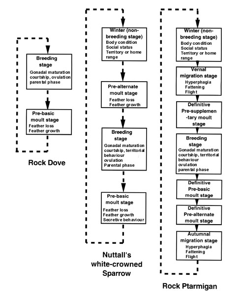
The life cycle of vertebrates is made up of a series of distinct stages each independent of the other, although they may overlap to varying degrees (Jacobs 1996; Wingfield et al. 1999). Some examples of life history stages are given in Fig. 1. Each box represents a distinct life history stage and they occur in a set sequence that cannot be reversed. For example, in the White-crowned Sparrow Zonotrichia leucophrys it is not possible to revert to pre-alternate (prenuptial) moult after the breeding season, the sequence must move on to the next stage, (pre-basic moult). This sequence of stages is the finite state machine of an individual's life history (Jacobs 1996). Sub-stages are unique to each stage and are expressed in many sequences and combinations within that stage (Jacobs 1996). For each organism we can postulate a finite state machine of a characteristic number of life history (phenotypic) stages that occur in a fixed sequence and usually on a schedule determined by such environmental phenomena as the changing seasons. Sub-stages, on the other hand, can occur on much more flexible schedules but only within their appropriate life history stage.
Presumably the number and sequence of life history stages, and the complexity of sub-stages within them, are genetically determined for each individual. However, the fine tuning of development and termination of a life history stage, and the combination of sub-stages expressed at any moment in a particular stage, are likely to be highly plastic. They should match local environmental and social conditions, and probably should be equally dependent upon experiential factors as well as environmental cues. Here we will address the finite state machine of life history stages as a whole and then focus on a specific stage - breeding - to explore possible ways in which experiential factors may act on a genetic framework to provide control mechanisms through neuroendocrine and endocrine secretions that orchestrate all aspects of reproduction.
Before we can discuss how an organism's life cycle may be influenced by genetic and/or experiential factors, an important question is how do we compare life history cycles with different degrees of complexity, i.e. numbers of stages and sub-stages? Although such issues have been addressed in terms of life history strategies, phenotypic plasticity etc., at the population level (e.g. West-Eberhard 1989), such issues within an individual as it adjusts life history stages and sub-stages to local conditions have been much less well studied (Jacobs 1996; Wingfield et al. 1997c, 1998, 1999).
Finite State Machines and Diversity Indices.
Transitions in morphology, physiological state and behaviour that make up the sequences of life history stages (i.e. finite state machines) involve periods of development of a life history stage followed by a 'mature capability' in which a number of sub-stages can then be activated. Hormones play a major role in development of each stage (and its termination) as well as activation of sub-stages. The mechanisms of these hormonal actions may differ markedly even if the same hormone is involved because the processes being regulated are different (e.g. territorial behaviour in different contexts, migration versus moult, catabolic or anabolic metabolism etc.). Each life history stage is independent of the others, although there may be overlap to varying degrees (Jacobs 1996). Some species may have more life history stages than others, and even within an individual, some life history stages may have a more complex set of sub-stages than others. The degree to which variation in life history stages exists is presented for three species of birds in Fig. 1.
The Rock Dove Columba livia has only two obvious life history stages, breeding and moult (from Johnston 1992), whereas Nuttall's White-crowned Sparrow Z. l. nuttallii has four (e.g. Blanchard 1941; Mewaldt & King 1977) and the Rock Ptarmigan Lagopus mutus has seven (Holder & Montgomerie 1992). Note also that the number of sub-stages within each stage varies. How do we compare the complexity of life history stages across taxa? Because these transitions of stage and activation of sub-stages are regulated by hormones there are likely to be major differences among species at cell and molecular levels. Additionally, it is highly likely that some aspects of this finite state machine are genetic and others experiential. Is it possible to analyse this diversity and develop appropriate hypotheses to test these questions? Ecologists have dealt with diversity issues such as these for many years and although this is still an active area of research, we can begin to apply these approaches to this conceptually similar problem, the diversity of life history stages and their sub-stages. As with species diversity, simple number of stages (cf species) may not be an accurate assessment of diversity because the duration (timing) of each stage is also critical. A number of questions arise that integrate all these possibilities and are derived from those questions posed by ecologists (e.g. Pielou 1969, 1975):
a). Why are there not more (or fewer) life history stages and will their durations be the same ? Another way of stating this would be, do the life history stages differ much in their tolerance ranges for environmental variables (see also Jacobs 1996).
b). Why are some stages widespread and others rare, and are their relative proportions (durations) constant ?
c). Are most, or all, of the life history stages within an individual fully adapted to the habitat at that time ?
From Fig. 1 we see that some organisms have only a few life history stages and others have many. Thus we can apply formulae for ecological diversity (e.g. species diversity indices) to finite state machines to give us a measure of finite state diversity. This allows us to go beyond simply counting numbers of life history stages, and indicates the diversity of stages as a function of their duration as well as number. Before finite state diversity can be measured, however, the temporal sequence of life history stages within an individual of a given population must be defined and applied equally to all (Jacobs 1996). This definition must specify the boundaries of the temporal sequence, how each stage is identified, and its duration measured. The boundaries of the temporal sequence could be defined at many levels such as day, month, tidal fluctuation, length of wet/dry seasons, year or longer. Numbers of life history stages must be determined by the same criteria in all populations. Jacobs (1996) defines a life history stage as having a unique set of sub-stages (i.e. not shared by other life history stages), and each life history stage occurs in a set temporal sequence that cannot be reversed. For example in the White-crowned Sparrow (Fig. 1), it is not possible to go back from the breeding stage to pre-alternate moult stage directly. It can only be attained by progressing through pre-basic moult and winter stages. On the other hand, the sub-stages within a life history stage can be activated in any sequence, or repeated many times within a life history stage (see below).
Duration of each life history stage can be measured directly from field observations. In the Rock Dove (Fig. 1), individuals are almost always in breeding condition once adult, as indicated by developmental state of the gonads. Pre-basic moult, on the other hand, may be restricted to a few months of the year (Johnston 1992). Thus, the durations of these two life history stages are very different but they also overlap almost completely. In the Rock Ptarmigan, a larger number of life history stages means shorter duration of each stage (Fig. 1) unless there is considerable overlap. In general, some life history stages (such as winter and moult) may be more compatible in terms of overlap whereas others such as migration and breeding are much less compatible (obviously it is not possible to build a nest and incubate eggs while covering long distances on migration). The application of diversity indices is one way by which we can describe number, duration and overlap of life history stages across all populations of all taxa.
Finite State Diversity
Bearing in mind the admonition of Pielou (1969; 1975) that we should be careful in how we apply mathematical techniques to biological problems, and not take too many liberties in stretching assumptions made in mathematics to highly complex biological processes, we have applied the Shannon diversity index to finite-state machines of life history stages. We adopt the ideas of MacArthur (1964) for species diversity to use this formula to calculate the diversity of life history stages as a function of their number, duration and degree of overlap. In this way we are able to formally describe finite state machines of different populations as a framework to formulate hypotheses about hormonal control. We feel that this objective method will allow us to identify which populations should be compared to give maximum power in determining those mechanisms.
When describing the diversity of biological communities ecologists found that simple species lists fail to account for the abundance of individual species. For example, a simple community may have four species of equal abundance, another may have four species in which one is common and the other three are rare. Do these communities have the same species diversity? Similarly we could apply these ideas to a finite state machine where the sequence of life history stages is analogous the community, with varying numbers of life history stages (cf species in a community), each with different durations (cf numbers of individuals of a species in a community). Over three decades ago, information theory provided a basis by which to describe species diversity in terms of number of species and the abundance of each. We propose here to follow the same procedures to compare finite state diversity of life history stages and their durations across taxa. In turn we feel that this framework may then allow us to compare mechanisms by which the sequence and expressions of life history stages are controlled, particularly in relation to genetic versus experiential factors.
Many mathematical methods have been employed to describe diversity, but one of the commonest is the Shannon Index (MacArthur & MacArthur 1961; MacArthur 1964):
H = - S pi loge pi
where H = diversity index and pi is the proportion of all individuals in the community that belong to species i. If all species in a community have equal abundance then the Shannon Index will be high, but if some species are more abundant than others then the Index will be lower. This method and others has been used by community ecologists to identify possible causes of variation in diversity in relation to habitat complexity (MacArthur & Preer 1962), latitude (Ricklefs 1987), competition and predation (Martin 1988), and disturbance (Connell 1978).
These techniques have also been applied to other areas of biology, for example, to describe and compare the length of birds' breeding seasons (Wyndham 1986). In some avian species the breeding season is constant from year to year (i.e. only one or two months in which nesting occurs) whereas in others the breeding season may be highly variable covering 10 months in one year and only two months in another (see also Wingfield et al. 1992, 1993). Thus simply comparing the number of months that nesting can occur in any one year for each population may be misleading. Wyndham (1986) used the Shannon Index to calculate the number of 'equally good months' for breeding from the formula above where pi is now the proportion of nests initiated in the i'th month. The number of 'equally good months' for breeding will vary from 1, when all nest are initiated (eggs laid) in one month in all years to 12, when the number of nests initiated is equal in all months of the year in each year. Wyndham (1986) points out that the number of 'equally good months' varies only as a function of the proportion of birds breeding in each month and does not differentiate between single and bimodal breeding seasons. Nevertheless, the calculation of the number of 'equally good months' for nesting allows a much more precise comparison of breeding seasons among species in relation to habitat, latitude etc. Application of these calculations to the breeding seasons of an australasian species, the Zebra Finch, Poephila guttata, shows a highly seasonal component to breeding (Zann et al. 1995). This species has long been considered a pure opportunist capable of breeding in any month in relation to unpredictable rains but, this analysis suggests that although the Zebra Finch is capable of breeding at any time year there is still an underlying seasonal component. It is likely that the control mechanisms for breeding in this species will be different than formerly supposed. Such an approach also allows us to choose populations with similar or very different values for 'equally good months' and then compare endocrine mechanisms experimentally.
Because the breeding season is a typical life history stage, it is reasonable to go one step further and apply this kind of analysis to other life history stages in a finite state machine. To illustrate these points we present some theoretical examples first as a way of defining our methods. The boundary of the temporal sequence we define here as one year with intervals of months (i.e. 12 intervals in Fig. 2). The vertical axis is then made up of different hypothetical life history stages (for example 6 stages in Fig. 2). For a given temporal sequence of hypothetical life history stages (the finite state machine) we can use the formula above to calculate the mean stage interval diversity (MSID), that is a measure of the diversity in duration of each life history stage; and the temporal stage diversity (TSD) which is a measure of the diversity of life history stages as a function of not only their number, but also duration and degree of overlap. Both of these measures may have considerable import for hormone mechanisms (see below). Some hypothetical examples will now show how MSID and TSD vary.
If we assume six life history stages each of two months duration (indicated by the shaded circles corresponding to each stage and interval in Fig. 2 upper panel) and with no overlap, then this gives us a MSID of 2 (i.e. all are the same - two months duration) and a TSD of 6 (there are 6 life history stages with no overlap). Note also that in these finite state machines, the organisms must be in at least one life history state at all times (otherwise it obviously would not be alive). If we then assume six life history stages with unequal duration (one to four months, Fig. 2 middle panel) then we get a MSID of 2.7 and a TSD of 4.5. In the lower panel of Fig. 2 we have six life history stages with an extremely skewed duration. One stage covers seven months (intervals) and the other 5 are of one month (interval) each with no overlap. In this case the MSID = 4.5 and TSD = 2.7. Clearly the diversity of life history stages is not simply a function of how many there are, but also a function of duration of each stage.
If we now go to our avian examples from Fig. 1 and apply the diversity indices, once again we see considerable variation (Fig. 3). In the Rock Dove the breeding stage is found in up to 10 months and the moult in six months. This gives a MSID of 8.5 (both are relatively long in duration) and a TSD of 1.3 (very few stages but this time with considerable overlap). Although there are two life history stages, because of variation in duration and overlap in timing, the TSD is less than 2. In the White-crowned Sparrow (mid panel of Fig. 3), the four life history stages are of shorter duration with no overlap giving a MSID of 3.8 and a TSD of 3.1. The Rock Ptarmigan (lower panel of Fig. 3) has seven life history stages with some degree of overlap. In this case, MSID = 2.4 and TSD = 4.9. Clearly the numbers, duration, and degree of overlap of life history stages need to be taken into account when describing the diversity of finite state machines. But, is this useful for deriving hypotheses to test mechanisms?
From these data it now becomes clear that although the application of the Shannon Index is useful for comparing finite state diversity across taxa, it has a potential drawback in that in some cases very different temporal sequences of life history stages can give similar MSID and TSD values. Exactly the same problems have been encountered by ecologists when using this formula, and others, to determine species diversity (Pielou 1969, 1975). For these reasons community ecologists have criticised this approach. However, we feel that this property of the method may indicate useful information. Here we use the technique to describe the finite state diversity not define it. Thus is it possible that although the number and temporal sequence of life history stages in some species may appear to be different superficially, the ratios of MSID and TSD values suggest they are very similar. Does this mean that the hormonal mechanisms underlying control of each stage are also similar? Are the control mechanisms more likely to be genetically pre-ordained and less influenced by experiential factors? Conversely we could argue that since the ratios of MSID to TSD of these species are similar, but very different from those of others, then the latter species may have different control mechanisms and different degrees of genetic versus experiential input for those control mechanisms. These hypotheses are eminently testable and will allow us to quickly identify extremes within taxa and similarities across widely diverse taxa. We can then test whether mechanisms differ or show convergence accordingly. This has the potential to provide a basic framework for environmental endocrinology.
Before going on we should also point out that we are aware that the Shannon Index should be ideally applied to an infinite population (or collection of stages and intervals, Pielou 1969, 1975). This is obviously not the case for finite state machines with limited numbers of life history stages and intervals in which they are likely to occur. We also calculated the Brillouin index for a finite population (Pielou 1969, 1975) and compared the MSID values using the two indices for finite state machines from several species and populations of species (Fig. 4). Because the MSID values using the Shannon Index and Brillouin index in relation to the number of life history stages are super-imposed and since the Brillouin index poses calculation problems owing to factorials within the formula, we use the Shannon Index throughout.
Finite State Diversity in Different Taxa
Natural histories for several species, and populations within species, are used to determine the number of life history stages and their estimated duration in months. From these data the MSID and TSD are calculated and plotted against the number of life history stages (Fig. 5). Species from which data are compiled are named in the legend to Fig. 5 with references. MSID decreases as the number of life history stages increases (Fig. 5, upper panel). This is expected as the duration of each stage must go down as the number of stages increases. However, this relationship is not a simple straight line because the degree of overlap of timing of life history stages may differ. There can be considerable variation in MSID for species with similar life history stages (e.g. stages 2 and 3 in the upper panel of Fig. 5). Similarly, there can be wide variation in life history stages for a particular MSID (e.g. see the range of stages for the MSID value of 3.5-4.5 in Fig. 5).
For TSD the trend is opposite as we would expect (lower panel of Fig. 5). As the number of life history stages increases then TSD should also increase but again this is not a perfect straight line. There is wide variation in TSD for species with identical numbers of life history stages (e.g. stage 5 in Fig. 5 lower panel). Additionally, TSD may be similar over a range of life history stages (e.g. TSD value of 1.5-2.5 in lower panel of Fig. 5). These data suggest that calculating TSD and MSID may tell us much about variation in finite state diversity for different species. Are the mechanisms underlying control of the temporal sequence of life history stages the same for MSID values of 10 and 4 when only two life history stages are expressed (e.g. Fig. 5 upper panel) or for TSD values of 4.5 and 1.5 when 5 phenotypic stages are expressed? Conversely, are the mechanisms underlying the regulation of transitions from stage to stage similar when MSID values are comparable across several species with different numbers of phenotypic stages? These kinds of comparisons can indicate the most critical experiments to determine how individuals orchestrate morphological, physiological and behavioural adjustments throughout their life cycles.
It should also be pointed out here that broad phylogenetic comparisons of species in this way may introduce spurious variation simply because many species are not closely related and may have evolved diverse life history stages that give rise to the wide range of MSID or TSD with similar numbers of life history stages. Comparisons of closely related species within a sub-family, e.g. the emberizinae (Fig. 6) show that the relationships of MSID, TSD and numbers of life history stages are more linear. This is even more striking if a single genus is compared (e.g. Zonotrichia, Fig. 7). Here then it is possible to conduct experiments on congeners to determine how mechanisms differ along a defined array of finite state diversities. If we now take examples of these closely related taxa with different diversity indices we can test whether the control mechanisms are more fixed, i.e. less subject to change, at one extreme or more influenced by experiential factors at the other extreme. For example, it could be argued that a population with a larger number of life history stages with little overlap would have less flexibility in timing and thus control mechanisms would be more rigidly genetic (endogenous) with environmental factors acting on a preordained programme. On the other hand, fewer life history stages with overlap would provide much greater flexibility of timing. Although there still may be an underlying genetic programme that provides context and sensitivity to appropriate environmental cues (e.g. Wingfield 1983), more experiential effects would allow 'fine-tuning' to local conditions. Analysis of finite state diversity in this way provides an objective way of considering not only the number of life history stages but also their durations and degree of overlap with other stages. Clear hypotheses can then be formulated and which populations will provide the best comparisons can be identified even among very closely related taxa.
Assessing the Complexity of Sub-stages Within Each Phenotypic Stage.
Each life history stage has a unique set of sub-stages (Fig. 1). Whereas life history stages are expressed in a fixed temporal sequence, the sub-stages can be expressed in a variety of sequences and/or sets. From Fig. 1 it is clear that the number of sub-stages within each life history stage can vary greatly from species to species and from stage to stage within an individual. Since the activation of these stages requires hormonal and neural input, probably in response to appropriate environmental cues, then the control mechanisms may vary from species to species within a type of stage as well as among different stages within an organism. Thus there is a need to formally analyse the degree of complexity of sub-stages within each life history stage. Not only the number of sub-stages, but also how each is connected to other sub-stages should be considered. This requires a different analysis from the finite state machine of life history stages partly because the expressed 'set' of sub stages at any point in a specific life history stage is the overall morphological, physiological and behavioural state of the organism at that time. This is dictated by a number of environmental and social factors that may vary within an individual from moment to moment, or among individuals in a population according to micro-habitats and experience. It is likely that control mechanisms for expression of sub-stages are dependent more on experiential factors but within limits defined by the finite state machine of life history stages that is largely genetically determined.
An illustration of variation in complexity of sub-stages is given in Fig. 8 for the migratory White-crowned Sparrow, Z.l. gambelii. The breeding life history stage (Fig. 8a) is complex and consists of at least eight distinct sub-stages. Firstly, gonad development is necessary and then several sub-stages can follow such as establishment of a breeding territory, courtship and pair-bonding, nest building, and ovulation/copulation/egg laying. Following this sexual phase then several parental sub-stages can be expressed such as incubation, feeding nestlings and fledging. There is a temporal sequence of these events in a broad sense, but note that if the nest or eggs are lost to a predator then the various sexual sub-stages can be expressed again. This is not possible for the finite state machine of life history stages (see above, Jacobs 1996). Also, if the population is multiple brooded then sexual and parental sub-stages can be repeated. This does not mean, however, that all sub-stages are equally connected with other sub-stages. In Figure 8a, we show the main known connections of sub-stages. The maximum number of connections for a given repertoire of sub-stages within a life history stage is calculated from the formula n(n-1). In Figure 8a the maximum number of connections possible is 56 but only 19 (ratio of 0.34) have been identified in field studies of White-crowned Sparrows (from Blanchard 1941; Blanchard and Erickson 1949; Mewaldt & King 1977; Wingfield & Farner 1978a,b).
The migration (vernal) life history stage is less complex (Fig. 8b) consisting of migratory readiness (zugdisposition) followed by periods of hyperphagia and fattening, and a transition period before an actual flight. After landing there is another transition back to hyperphagia and fattening for the next leg of migration (see Wingfield et al. 1990). Here the maximum number of connections is 20 but only 8 (ratio of 0.4) are demonstrated (Fig. 8b). For the pre-basic moult stage (Fig. 8c) there are only three sub-stages and the ratio of connections observed to possible is 0.5. For the winter life history stage there is also a small number of sub-stages but connectivity is maximal (i.e. the ratio is 1.0, Fig. 8d). Connectivity varies not only as a function of the number of sub-stages but also as a function of known relationships and sequences of events within a life history stage.
We can also compare sub-stages within the same life history stage across different taxa. For example, the connections of sub-stages in the breeding stage are different depending upon whether the species is single-brooded (Fig. 9a) or double brooded (Fig. 9b). The potential number of connections is 56 in each case, but the number of actual connections is 16 (ratio of 0.29, Fig. 9a) for single brooded species and 19 (ratio of 0.34, Fig. 9b) for double-brooded species. For a brood parasite (e.g. the Brown-headed Cowbird, Molothrus ater, Dufty & Wingfield 1986a,b) there is no parental phase at all because females lays eggs in the nests of other species. Here there are only 4 sub-stages in the breeding life history stage (Fig. 9c) with a connectivity of 0.5. One can also compare individuals within a population but with different breeding life history stages (Fig. 10). Breeding females that show parental care will have a connectivity ratio of about 0.34 (Fig. 10a and as in Fig. 8a and Fig 9a). However, many males show no parental behaviour and thus have a more limited number of sub-stages with a connectivity of 0.58 (Fig. 10b). In some cooperatively breeding species such as the White-browed Sparrow Weaver, Plocepasser mahali, (Wingfield et al. 1991) there is a dominant male and a dominant female who have both a sexual phase and provide parental care (connectivity thus equals 0.34 as in Fig. 10a). But, there are also other individuals in the group that have no sexual phase but do feed young (Fig. 10c) and are called 'helpers-at-the-nest'. Here there are only 4 sub-stages in the breeding life history stage with a connectivity of 0.5. These variations in numbers of sub-stages within the same life history stage of individuals within a population and their connectivity may have fundamental influences on the neural and hormonal control mechanisms. More complex sets of sub-stages within a life history stage with higher degrees of connectivity may require much more plasticity in control mechanisms with experiential, especially learning, components being important. Life history stages with fewer sub-stages or lower connectivity may still be plastic but on a reduced scale in which learning and experience play a lesser role. In both scenarios it is reasonable to assume that a preordained genetic programme regulates development of the life history stage so that the repertoire of sub stages can be expressed. Thus experiential effects, including learning, probably are dependent to varying degrees on an underlying genetic base. Such analysis may allow more meaningful comparisons to be made when conducting experiments to determine control mechanisms.
Implications for hormone control mechanisms
Endocrine secretions regulate many aspects of homeostasis as well as transitions in morphology, physiology and behaviour in relation to predictable changes in the environment. Since most vertebrates live in changing environments, they change their state to maximise survival at different times of year. However, the number of life history stages, their durations, and the degree of overlap with other stages, varies from species to species and from population to population. As hormones regulate the development of each stage and its termination, then the number of stages and the degree of overlap with other stages could have a major influence on neuroendocrine and endocrine mechanisms and their control by environmental cues. For example, the need for accurate timing of the transitions from one stage to the next in Ptarmigan may be more important than in the Rock Dove because of different degrees of diversity in the stages (Fig. 1 and Fig. 3). It is known that annual changes in photoperiod acting through neuroendocrine and endocrine secretions regulate at least some of the life history stages of Rock Ptarmigan (e.g. Stokkan et al. 1986, 1988). On the other hand, regulation of breeding and moult appear to be independent of photoperiod in the Rock Dove (Lofts & Murton 1968). Diversity indices thus may help identify where possible differences, or similarities, in environmental and endocrine mechanisms may exist.
Each stage has a unique set of sub-stages that can be activated in complex sequences or combinations. Analysis of connectivity allows us to compare not only number of sub-stages, but also the complexity of interrelationships of that set of sub-stages. For example in Fig. 10 we can see that the neuroendocrine and endocrine mechanisms activating sexual sub-stages in a co-operative breeder, the White-browed Sparrow Weaver, may be in operation in dominant breeding males and females, but not necessarily in helpers-at-the-nest that only express parental sub-stages. Does this mean that the helpers are incapable of expressing sexual sub-stages, or just lack necessary stimuli to activate them? In another co-operative breeder, the Florida Scrub Jay, Aphelocoma coerulescens, helpers-at-the-nest that usually express only parental behaviour and do not breed themselves can, given the chance such as a vacant territory, breed and show the full repertoire of sexual behaviour (Schoech et al. 1996). Furthermore, if female Florida Scrub Jay helpers are given oestradiol implants to activate sexual behaviour, a helper male may pair with them and breed (Schoech et al. 1996). On the other hand, it appears that brood parasites such as the Brown-headed Cowbird can activate sexual sub-stages (Fig. 9), but have lost the ability to express parental sub-stages even if given hormones known to activate parental behaviour in other species (Dufty & Wingfield 1986a,b). This suggests that the genetic control of reproductive processes in Brown-headed Cowbirds can no longer activate parental behaviour regardless of hormone input or experience.
Clearly, not all sub-stages within a stage must be expressed, but only when appropriate and as signalized by environmental and social cues. In some populations, certain sub-stages may have been lost emphasising the presence of an underlying genetic programme that ultimately regulates when and if a specific sub-stage may be expressed. Other comparisons across life history stages show that sub-stages are truly unique to their life history stage. For example, in Song Sparrows, Melospiza melodia, males in the non-breeding stages of autumn and winter (c.f. Fig. 1) were unable to respond with sexual sub-stages typical of the breeding stage (c.f. Fig. 1) when presented with females made sexually receptive in the winter by experimental treatment with oestradiol. However, these males responded normally once increasing photoperiod triggered development of the breeding stage in spring (Wingfield & Monk 1994). Analysis of finite state diversity may allow comparisons of these types to be made and determine genetic versus experiential effects on reproductive and other stages in the life cycle of vertebrates.
Classifying environmental signals that affect control mechanisms
There is a vast literature on the responses of vertebrates to environmental signals, but despite the apparent hopeless complexity of cues and responses, the environmental information used by animals can be organised into four major types, based on the major effects of these signals (Wingfield 1983; Wingfield & Kenagy 1991). The first group, called 'initial predictive information', is a type of signal that provides very reliable long term predictive information so that an individual can begin preparing for a future event several weeks or even months in advance. For example, it is well known that the seasonal change in day length can act as a signal to promote gonadal development in anticipation of the breeding season. These long term predictive cues are then integrated with the second group of environmental signals called 'supplementary factors' that provide short term predictive information. In most habitats, there is temporal variation in predictive events. For example, at mid-latitudes some springs are early and warm, others are late and cool. Therefore individuals need to fine tune changes in reproductive function induced by initial predictive information to give maximum fitness. Examples of supplementary cues are local temperature, availability of food, nest sites, rainfall, etc. Integration of changes of reproductive state in response to predictable fluctuations of the environment are co-ordinated precisely by these two types of signals.
The third group of environmental factors is called 'integrating and synchronising information'. This group comprises all of the behavioural interactions, inter- and intra-sexual, among groups, and between adults and young. They serve to integrate changes in behaviour with reproductive state, and also synchronise the behaviour of a breeding pair or group during nesting (Wingfield & Moore 1987; Wingfield et al. 1994). A great deal of research over the past fifty years indicates that integrating and synchronising information impinges upon all aspects of an animal's life. However, the critical importance of social influences and the profound implications for an individual's physiology have not been appreciated fully. The fourth class of environmental cues is called 'modifying information' or labile perturbation factors (e.g. Wingfield et al. 1998), and will not be further addressed here.
We use mathematical techniques such as log-linear analysis, information theory and spectrum analysis to model whether individuals should integrate predictive environmental signals or rely more heavily upon one or the other (Wingfield et al. 1992, 1993). For example, if a future event is highly predictable and restricted in time, then only one reliable environmental cue is needed to trigger appropriate preparation. On the other hand if a future event is much less predictable, the animal should monitor and respond to more environmental cues to co-ordinate precise adjustment of reproductive state with changing environment. Using the predictability of a given habitat, we can calculate an 'environmental information factor' (Ie). This factor reflects the degree to which a species within that habitat should use available environmental cues to regulate gonadal development and onset of breeding. If the Ie factor is low, individuals should focus on one or very few reliable cues (e.g. photoperiod), whereas a high Ie predicts that individuals should be sensitive to many environmental cues to make appropriate adjustments in their reproductive schedules (Wingfield et al. 1992, 1993). Research to date (e.g. Wingfield et al. 1996, 1997a) has shown this to be a powerful tool. Simple demographic data (e.g. timing of breeding from egg-laying dates) and field endocrine data provide bases from which to test these models further. Mechanisms by which the brain transduces such information can then be compared in populations that represent different extremes of responsiveness. The endocrine pathways by which this information is then passed on to specific tissues, and how those tissues respond, can also be investigated.
Three Phases of Reproductive Development.
It has now become clear that reproductive development in birds can be separated into three distinct phases probably with different control mechanisms. In the first phase, development of the breeding stage, the gonads grow from an immature state to near functional capacity (mature capability of the stage). The second phase involves rapid final maturation of ovarian follicles (yolk deposition) culminating in ovulation and oviposition (i.e. onset of the breeding stage). In contrast, the testes progress to functional maturity without a pause. Thus these phases are distinct in females but not in males. Finally, the breeding stage is terminated when the gonads regress back to a non-functional state and the next life history stage takes over. The photoperiodic control (initial predictive information) of the first phase has received many decades of attention (e.g. Farner & Follett 1979; Nicholls et al. 1988). However, integration of supplementary information as well as variations in responsiveness to these specific cues seen among populations has not been well studied (see Wingfield et al. 1992; 1993). How these cues may influence the two phases of ovarian development, as well as termination of the breeding stage are even less well known.
Photoperiodic regulation of the first phase of reproductive development involves increased secretion of chicken gonadotrophin-releasing hormone 1 (cGnRH-1), the major GnRH in passerines (Sherwood et al. 1987). This then regulates release of the gonadotrophins luteinizing hormone (LH) and follicle-stimulating hormone (FSH) that in turn orchestrate gonadal growth and secretion of sex steroid hormones. The latter then trigger development of secondary sex characters and reproductive behaviour (see Wingfield & Farner 1993 for a review of wild birds). Increased levels of gonadotrophins in blood are accompanied by elevated LHß-subunit mRNA titers in the anterior pituitary, and a rise in LH and FSH receptors in the testes of Z.l. gambelii (Ishii & Farner 1976; Kubokawa et al. 1994). In females, photoperiodic cues trigger release of the same reproductive hormones and ovarian maturation follows, but only to a sub-functional level (e.g. King et al. 1966; Wingfield and Farner 1980). In Zonotrichia, this rapid first phase of ovarian growth culminates when follicles are about 2-3 mm in diameter and contain white-yolk only. Females generally will not progress beyond this phase unless the environment is conducive to nesting (King et al. 1966). A second set of supplementary factors (or inhibitors) regulates the next phase, rapid deposition of yellow yolk (under the control of oestradiol secretion) and egg-laying (Wingfield & Farner 1980). The interaction of initial predictive information (probably largely genetic) and supplementary information (probably largely experiential on a preordained genetic programme) provide varying degrees of plasticity in the timing and integration of reproductive processes.
Effects of Temperature.
Temperature is one supplementary factor known to modulate gonadal maturation in both phases. Mathematical models of egg-laying dates in sparrows indicated that species with a low Ie factor should be insensitive to supplementary environmental cues such as temperature and be driven primarily by photoperiod. Experimental results were consistent with these predictions (Wingfield et al. 1996, 1997a). Z.l. pugetensis, a species with a high Ie factor, showed effects of increasing temperature on testicular and ovarian maturation in the first phase. Furthermore, in females, exposure to 30°C resulted in deposition of yellow yolk and rapid final maturation of the ovary indicating onset of the second phase. In contrast, Z.l. gambelii, a species with a low Ie, did not show these responses. This suggests that the latter taxon is largely driven by photoperiod with little flexibility in timing whereas the former taxon has greater plasticity in timing and integration of reproductive processes. Whether this may reflect varying degrees of genetic and experiential input could be tested in the future.
Although photoperiodically-induced rises in gonadotropins are mediated through the stimulation of cGnRH-1 from hypothalamic neurons (e.g. Follett 1984; Nicholls et al. 1988), the mechanisms by which temperature modulates this response remain unclear. In Z.l. pugetensis, we find no changes in plasma levels of LH or FSH in either sex despite profound effects on gonadal maturation in both phases (Wingfield et al. 1997a). These data suggest that temperature cues are signalized through a pathway other than the GnRH - gonadotrophin axis. We have considered two alternatives: thyroid hormones and glucocorticosteroids. Low temperature does not increase circulating levels of thyroxine (T4) or tri-iodothyronine (T3). Thus it is unlikely that temperature effects on the first phase of gonadal maturation are mediated through the hypothalamo-pituitary-thyroid axis. Nor is it likely that the stress of low temperature is the mechanism that retards gonadal growth because plasma levels of corticosterone (an indicator of stress - e.g. Wingfield et al. 1998) are similar in all groups. Our current hypothesis is that some other factor mediates the effect of temperature, presumably at the level of the gonad (e.g. gonadotrophin receptors), since plasma levels of gonadotrophins (and presumably GnRH) are unaffected. Similarly, how temperature affects the second phase of ovarian maturation is unclear. Identical data have been obtained for male and female Z.l. oriantha and Melospiza melodia morphna, both of which have high Ie's (Wingfield et al. unpublished), suggesting a true phenomenon and not a chance occurrence.
Effects of Social Cues.
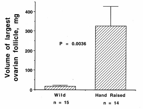
It is well known that the presence of the opposite sex can enhance photoperiodically-induced gonadal maturation in both phases (see Wingfield et al. 1994 for review). Experiments on Z.l. pugetensis in show that isolation of females from males abolishes temperature effects on the second phase of ovarian maturation. Social cues and temperature may interact to regulate both phases of gonadal maturation (Wingfield et al. 1997). It is also well known that behaviour of sexually mature males can hasten ovarian development and sexual behaviour of females accelerates testicular development (see Wingfield et al. 1994 for extensive review). However, there is also growing evidence that experience may play a major role. Female Song Sparrows raised in captivity show much greater ovarian development and even lay eggs the following breeding season. Wild caught females of the same age brought into captivity after they become independent of their parents show much less ovarian development on the same conditions in captivity (see Fig. 11). These data clearly indicate a great effect of experience super-imposed on a genetic programme of gonadal development triggered by initial predictive cues such as increasing day length.
Effects of Food.
Availability of food, quality of nutrition, and endogenous reserves of fat and protein can have profound influences on reproductive function (see Follett 1984). However, the mechanisms by which food supply acts as supplementary information remain equivocal (Wingfield & Kenagy 1991). Many experiments have been done, but they may not be relevant to an individual in its natural environment since severe food restriction (i.e. nutritional stress) is often the experimental paradigm (Wingfield & Kenagy 1991). There appears to be a seasonal component to the Red Crossbill Loxia curvirostra reproductive cycle, probably regulated by photoperiod, that brings the birds into breeding condition in July. There is another potential reproductive period in winter that is entirely opportunistic (Hahn 1995), controlled by factors other than day length and temperature (since the latter is at a seasonal low in January). A regulatory role of food supply is unlikely to be simply caloric intake since captive Crossbills with ad libitum food fail to breed in winter. Photostimulated male Crossbills fed a laboratory diet equal to what they normally would eat on short days, show similar testicular growth to males fed ad libitum, and much greater development than males held on short days (Hahn 1995). After food-restricted males on long days are given food ad libitum, testicular development is significantly greater than in males that have continuous access to ad libitum food. These exciting data suggest that perception of food availability may affect gonadal development. Body mass and food intake are similar among groups regardless of availability of food.
CONCLUSIONS
There is perhaps as much diversity in the life history cycles of organisms as there is diversity in species themselves. This poses an enormous problem as to how biologists might study such diversity, determine the degree to which genetics, phenotypic plasticity and experience (including learning) interact to give diversity of life histories, and then determine the mechanisms at a more reductionist level. For a mechanistic biologist it is particularly difficult to deal with such a degree of diversity. However, we need to go beyond focusing on a single population of individuals and look at a broader picture at community and even global levels. He we have outlined possible ways in which we can look at diversity of life history stages across taxa and develop specific hypotheses that are aimed at probing possible mechanisms. Tests of these hypotheses are only just beginning but the results to date suggest that this approach has at least heuristic value in exploring how we might come to grips with such diversity. Finite state machine theory reduces the life history cycles of vertebrates to a sequence of life history stages occurring on a temporal scale that is fixed to varying degrees depending upon the taxon and population. The sequence is probably the result of an endogenous (genetic) programme and each life history stage provides context in which a combination of unique sub-stages can be activated by experiential factors. Once the life history cycle progresses to the next stage, then a whole new set of sub-stages become possible, and the set of sub-stages from the previous life history stages can no longer be expressed. There may be varying degrees of overlap of some stages, but this is usually limited (see below). Thus, experiential factors determine combinations of sub-stages that give morphological, physiological and behavioural state at that time. This plasticity is restricted within the bounds of each life history stage determined by the underlying genetic programme. We incorporate ideas that community ecologists have used for decades to analyse the finite state machine of life history stages to indicate which comparisons of taxa and populations are most appropriate to test hypotheses generated.
When considering endocrine control mechanisms as well as the degree of genetic programming that may underlie the expression of the finite state machine of life history stages, it is important to remember there are certain constraints to the system. There are limits to the number of life history stages that can be expressed simultaneously simply because each has a certain 'cost' in terms of energetics. Too many stages expressed at the same time may be too costly and serve to reduce inclusive fitness. Breeding and moult life history stages are often regarded as mutually exclusive in many north temperate avian species (e.g. Wingfield & Farner 1980, 1993). A combination of reproduction, moult and migration would be obviously detrimental. It may be thus more adaptive to express life history stages in discrete temporal sequences in which overlap is reduced. However, this in itself introduces an additional constraint, because more life history stages with reduced overlap means the duration of each stage within a life cycle must also be reduced. Since each stage has a development and termination period, there is clearly a limit to how many may be expressed within a year. Moreover, more life history stages also mean less flexibility in timing. Whether this is reflected in selection for genetic programmes that drive a sequence of life history stages with little plasticity to accommodate experiential factors remains to be seen but could be tested. Conversely, few life history stages allows longer duration, more overlap (with less 'cost') and may lead to a genetic programme with much greater flexibility of timing and thus sensitivity to experiential factors.
Now that we have a theoretical framework to assess finite state diversity among many taxa, it may be possible to search for common mechanisms, determine to what extent experiential factors depend upon an underlying genetic programme, and to what degree populations in different habitats have plasticity in the system to deal with environmental change.
ACKNOWLEDGEMENTS
Much of research conducted in the investigations cited here were supported by grants from the Office of Polar Progams, and the Division of Integrative and Behavioural Neurobiology from the National Science Foundation to JCW. Wingfield is also grateful for support from the Benjamin Meaker Fellowship (University of Bristol), a John Simon Guggenheim Fellowship, and a Russell F. Stark University Professorship (University of Washington). The authors are also grateful to Professor R. T. Paine for his advice and suggestions on comparing diversity of life history stages across species.
REFERENCES
Anderson, D.J. 1992. Masked Booby. In: Poole, A., Stettenheim, P. & Gill, F. (eds) The Birds of North America: Vol. 2, No. 73, 16 pp. Philadelphia: Academy of Natural Sciences.
Blanchard, B.D. 1941. The white-crowned sparrows (Zonotrichia leucophrys) of the Pacific seaboard: environment and annual cycle. University of California Publications in Zoology 46:1-178.
Blanchard, B.D. & Erickson, M.M. 1949. The cycle in the Gambel sparrow. University of California Publications in Zoology 47: 255-318.
Briskie, J.V. 1992. Smith's Longspur. In: Poole, A., Stettenheim, P. & Gill, F. (eds) The Birds of North America: Vol. 1, No. 34, 16 pp. Philadelphia: Academy of Natural Sciences.
Cabe, P.R. 1992. European Starling. In: Poole, A., Stettenheim, P. & Gill, F. (eds) The Birds of North America: Vol. 2, No. 48, 24 pp. Philadelphia: Academy of Natural Sciences.
Chapin, J.P. 1954. The calendar of wideawake fair. Auk 71: 1-15.
Connell, J.H. 1978. Diversity in tropical rain forests and coral reefs. Science 199: 1302-1310.
Dufty, A.M.Jr. & Wingfield, J.C. 1986a. Temporal patterns of circulating LH and steroid hormones in a brood parasite, the brown headed cowbird, Molothrus ater. I. Males. Journal of Zoology (London) 208: 191-203.
Dufty, A.M.Jr. & Wingfield, J.C. 1986b. Temporal patterns of circulating LH and steroid hormones in a brood parasite, the brown headed cowbird, Molothrus ater. II. Females. Journal of Zoology (London) 208: 205-214.
Farner, D.S. & Follett, B.K. 1979. Reproductive periodicity in birds. In: Barrington, E.J.W. (ed.) Hormones and Evolution: 829-872. New York: Academic Press.
Follett, B.K. 1984. Birds. In: Lamming, G.E. (ed.) Marshall's Physiology of Reproduction 1. Reproductive cycles of vertebrates: 283-350. Edinburgh: Churchill-Livingstone.
Gratto-Trevor, C.L. 1992. Semipalmated Sandpiper. In: Poole, A., Stettenheim, P. & Gill, F. (eds) The Birds of North America: Vol. 1, No. 6, 20 pp. Philadelphia: Academy of Natural Sciences.
Hahn, T.P. 1993. Ph.D. Thesis, University of Washington.
Hahn, T.P. 1995. Integration of photoperiodic and food cues to time changes in reproductive physiology by an opportunistic breeder, the red crossbill, Loxia curvirostra (Aves; Carduelinae). Journal of Experimental Zoology 272: 213-226.
Holder, K. & Montgomerie, R. 1992. Rock Ptarmigan. In: Poole, A., Stettenheim, P. & Gill, F. (eds) The Birds of North America: Vol. 2, No. 51, 24 pp. Philadelphia: Academy of Natural Sciences.
Ishii, S. & Farner, D.S. 1976. Binding of follicle-stimulating hormone by homogenates of testes of photostimulated white-crowned sparrows, Zonotrichia leucophrys gambelii. General and Comparative Endocrinology 30: 443-450.
Jacobs, J. 1996. Regulation of Life History Stages Within Individuals in Unpredictable Environments. Ph.D. Thesis, University of Washington.
Johnston, R.F. 1992. Rock Dove. In: Poole, A., Stettenheim, P. & Gill, F. (eds) The Birds of North America: Vol. 1, No. 13, 16 pp. Philadelphia: Academy of Natural Sciences.
King, J.R., Follett, B.K., Farner, D.S. & Morton, M.L. 1966. Annual gonadal cycles and pituitary gonadotropin in Zonotrichia leucophrys gambelii. Condor 68: 476-487.
Kubokawa, K., Ishii, S. & Wingfield, J.C. 1994. Effect of day length on luteinizing hormone §-subunit mRNA and subsequent gonadal growth in the white-crowned sparrow, Zonotrichia leucophrys gambelii. General and Comparative Endocrinology 95: 42-51.
Lofts, B. & Murton, R.K. 1968. Photoperiodic and physiological adaptations regulating avian breeding cycles and their ecological significance. Journal of Zoology (London) 155: 327-394.
Lowther, P.E. & Cink, C.L. 1992. House Sparrow. In: Poole, A., Stettenheim, P. & Gill, F. (eds) The Birds of North America: Vol. 1, No. 12, 20 pp. Philadelphia: Academy of Natural Sciences.
MacArthur, R.H. 1964. Environmental factors affecting species diversity. American Naturalist 98: 387-397.
MacArthur, R.H. & MacArthur, J.W. 1961. On bird species diversity. Ecology 42: 594-598.
MacArthur, R.H. & Preer, J. 1962. On bird species diversity II. Prediction of bird census from habitat measurements. American Naturalist 96: 167-174.
Manuwal, D.A. & Thoresen, A.C. 1992. Cassin's Auklet. In: Poole, A., Stettenheim, P. & Gill, F. (eds) The Birds of North America: Vol. 2, No. 50, 20 pp. Philadelphia: Academy of Natural Sciences.
Martin, T.E. 1988. Processes organizing open-nesting bird assemblages: competition or predation ? Evolutionary Ecology 2: 37-50.
Mewaldt, L.R. & King, J.R. 1977. The annual cycle of white-crowned sparrows (Zonotrichia leucophrys nuttallii) in coastal California. Condor 79: 445-455.
Miller, A.H. 1962. Bimodal occurrence of breeding in an equatorial sparrow. Proceedings of the National Academy of Sciences U.S.A. 48: 396-400.
Mueller, A.J. 1992. Inca Dove. In: Poole, A., Stettenheim, P. & Gill, F. (eds) The Birds of North America: Vol. 1, No. 28, 12 pp. Philadelphia: Academy of Natural Sciences.
Nicholls, T.J., Goldsmith, A.R. & Dawson, A. 1988. Photorefractoriness in birds and comparison with mammals. Physiological Reviews 68: 133-176.
Pielou, E.C. 1969. An Introduction to Mathematical Ecology. Wiley Interscience, New York, 286 pp.
Pielou, E.C. 1975. Ecological Diversity. Wiley Interscience, New York, 165 pp.
Ricklefs, R.E. 1987. Community diversity: relative roles of local and regional processes. Science 235: 167-171.
Romero, L.M., Soma, K.K., O'Reilly, K.M., Suydam, R. & Wingfield, J.C. 1998. Hormones and territorial behavior during breeding in snow buntings (Plectrophenax nivalis): an arctic-breeding songbird. Hormones and Behavior 33: 40-47.
Schoech, S.J., Mumme, R.L. & Wingfield, J.C. 1996. Delayed breeding in the cooperatively breeding Florida scrub-jay (Aphelocoma coerulescens): inhibition or the absence of stimulation. Behavioral Ecology and Sociobiology 39: 77-90.
Sherwood, N., Wingfield, J.C., Ball, G.F. & Dufty, A.M. Jr. 1988. Identity of GnRH in passerine birds: comparison of GnRH in song sparrow (Melospiza melodia) and starling (Sturnus vulgaris) with 5 vertebrate GnRHs. General and Comparative Endocrinology 69: 341-351.
Stokkan, K.-A., Sharp, P.J., Dunn, I.C. & Lea, R.W. 1988. Endocrine changes in photo-stimulated willow ptarmigan (Lagopus lagopus lagopus) and Svalbard ptarmigan (Lagopus mutus hyperboreus). General and Comparative Endocrinology 70: 169-177.
Stokkan, K.-A., Sharp, P.J. & Unander, S. 1986. The annual breeding cycle of the high arctic Svalbard ptarmigan (Lagopus mutus hyperboreus). General and Comparative Endocrinology 61: 446-451.
West-Eberhard, M.L. 1989. Phenotypic plasticity and the origin of diversity. Annual Review of Ecology and Systematics 20: 249-278.
Whittow, G.C. 1992. Laysan Albatross. In: Poole, A., Stettenheim, P. & Gill, F. (eds) The Birds of North America: Vol. 2, No. 66, 20 pp. Philadelphia: Academy of Natural Sciences.
Wingfield J.C. 1983 Environmental and endocrine control of reproduction: an ecological approach. In: Mikami S.-I. & Wada M. (eds) Avian Endocrinology: Environmental and Ecological Aspects: 205-288. Tokyo and Berlin: Japanese Scientific Societies Press and Springer-Verlag.
Wingfield, J.C., Breuner C., Jacobs J.D., Lynn S., Maney D.L., Ramenofsky, M. & Richardson R. 1998. Ecological Bases of Hormone-behavior Interactions: the 'Emergency Life History Stage'. American Zoologist 38: 191-206.
Wingfield, J.C. & Farner, D.S. 1978a. The endocrinology of a naturally breeding population of the white-crowned sparrow (Zonotrichia leucophrys pugetensis). Physiological Zoology 51: 188-205.
Wingfield, J.C. & Farner, D.S. 1978b. The annual cycle in plasma irLH and steroid hormones in feral populations of the white-crowned sparrow, Zonotrichia leucophrys gambelii. Biology of Reproduction 19: 1046-1056.
Wingfield, J.C. & Farner, D.S. 1980. Environmental and endocrine control of seasonal reproduction in temperate zone birds. Progress in Reproductive Biology 5: 62-101.
Wingfield, J.C., & Farner, D.S. 1993. The endocrinology of feral species. In: Farner, D.S., King, J.R. & Parkes, K.C. (eds) Avian Biology: 9: 163-327. New York: Academic Press.
Wingfield, J.C. & Hahn, T.P. 1994. Testosterone and territorial behaviour in sedentary and migratory sparrows. Animal Behaviour 47: 77-89.
Wingfield, J.C., Hahn, T.P. & Doak, D. 1993. Integration of environmental cues regulating transitions of physiological state, morphology and behavior. In: Sharp, P.J. (ed.) Avian Endocrinology:111-122. Bristol: J. Endocrinology Ltd.
Wingfield J.C., Hahn T.P., Wada M., Astheimer L.B. & Schoech S. 1996. Interrelationship of day length and temperature on the control of gonadal development, body mass and fat depots in white-crowned sparrows, Zonotrichia leucophrys gambelii. General and Comparative Endocrinology 101: 242-255.
Wingfield J.C., Hahn T.P., Wada M. & Schoech S. 1997a. Effects of day length and temperature on gonadal development, body mass and fat depots in white-crowned sparrows, Zonotrichia leucophrys pugetensis. General and Comparative Endocrinology 107: 44-62.
Wingfield, J.C., Hahn, T.P., Levin, R. & Honey, P. 1992. Environmental predictability and control of gonadal cycles in birds. In: Grier, H. & Cochran, R. (eds) Biology of the Chordate Testis. J. Exp. Zool. Lond. 261: 214-231.
Wingfield, J.C., Hegner, R.E. & Lewis, D. 1991. Circulating levels of luteinizing hormone and steroid hormones in relation to social status in the cooperatively breeding white-browed sparrow weaver, Plocepasser mahali. Journal of Zoology London 225: 43-58.
Wingfield, J.C., Hillgarth, N., & Jacobs, J. 1997b. Ecological constraints and the evolution of hormone-behavior interrelationships. Proceedings of the New York Academy of Sciences 807: 22-41.
Wingfield J.C., Jacobs, J.D., Tramontin, A., Perfito, N., Meddle, S., Maney, D.L. & Soma, K. 1999. Toward an ecological basis of hormone-behavior interactions. In: Schneider, J. and Wallen, K. (eds) Reproduction in Context. Cambridge, Massachusetts, M.I.T. Press (in press).
Wingfield J.C. & Kenagy G.J. 1991. Natural regulation of reproductive cycles. In: Schreibman M. & Jones R.E. (eds) Vertebrate Endocrinology: Fundamentals and Biomedical Implications: Vol. 4, Part B: 181-241. New York: Academic Press.
Wingfield, J.C. & Monk, D. 1994. Behavioural and hormonal responses of male song sparrows to oestrogenized females during the non-breeding season. Hormones and Behavior 28: 146-154.
Wingfield J.C. & Moore M.C. 1987. Hormonal, social, and environmental factors in the reproductive biology of free-living male birds. In: Crews D. (ed.) Psychobiology of Reproductive Behaviour: An Evolutionary Perspective: 149-175. New Jersey: Prentice Hall.
Wingfield, J.C., Newman, A., Hunt, G.L.Jr. & Farner, D.S. 1982. Endocrine aspects of female-female pairing in the western gull (Larus occidentalis wymani). Animal Behaviour 30: 9-22.
Wingfield, J.C., Schwabl, H. & Mattocks, P.W.Jr. 1990. Endocrine mechanisms of migration. In: Gwinner, E. (ed.) Bird Migration: 232-256. Berlin: Springer-Verlag.
Wingfield J.C., Whaling C.S. & Marler, P.R. 1994. Communication in vertebrate aggression and reproduction: The role of hormones. In: Knobil E. & Neill, J.D. (eds) Physiology of Reproduction, Second Edition: 303-342. New York: Raven Press.
Wyndham, E. 1986. Length of birds' breeding seasons. American Naturalist 128: 155-164.
Zann, R.A., Morton, S.R., Jones, K.R. & Burley, N.T. 1995. The timing of breeding by zebra finches in relation to rainfall in central Australia. Emu 95: 208-222.
Fig. 1. Finite state machines of life history stages for three avian species. In the Rock Dove (Columba livia) there are two major life history stages, breeding and moult, designated by the boxes. Dashed lines indicate the direction of progression from one stage to another. Note also that the number of sub-stages (finer print within boxes) is greater for the breeding stage than for pre-basic moult. The centre column represents four life history stages for the Nuttall's White-crowned Sparrow (Zonotrichia leucophrys nuttallii). Again, dashed lines and arrows indicate the direction of progression. This temporal sequence cannot be reversed. Finer print within boxes indicates the number of sub-stages. On the right is the most complex finite state machine with seven life history stages in the Rock Ptarmigan (Lagopus mutus). Many, but not all, populations of Rock Ptarmigan are short distance migrants within the Arctic. Dashed lines and arrows indicate the direction of progression, and finer print in boxes represents the sub-stages. Sub-stages in the three different moult stages here have been omitted but include feather loss and feather growth in each case. These may be different for each type of moult because different feathers may be moulted, and even if they are in the same feather tracts, the colour of the feather that develops is different. So although the sub-stages in these different life history stages appear to be the same, they may in fact have very different ecological bases and control mechanisms (see Wingfield et al. 1996 for discussion of other examples).
Fig. 2. Schematic representation of finite state diversity. Each column represents an interval in a temporal sequence of hypothetical life history stages. In this example the intervals are months in a year. The rows represent hypothetical life history stages, for example we have six. The shaded circles indicate in which interval each life history stage is expressed by an organism in a given population. In the top panel, each stage has a duration of 2 months and there is no overlap. In this case the mean stage interval diversity (MSID) is calculated as 2 and the temporal stage diversity (TSD) is 6. In the middle panel the durations of stages vary giving a MSID of 2.7 and TSD of 4.5. In the lower panel, the duration of one stage seven months and the others are one month long each. MSID now equals 4.5 and the TSD is 2.7.
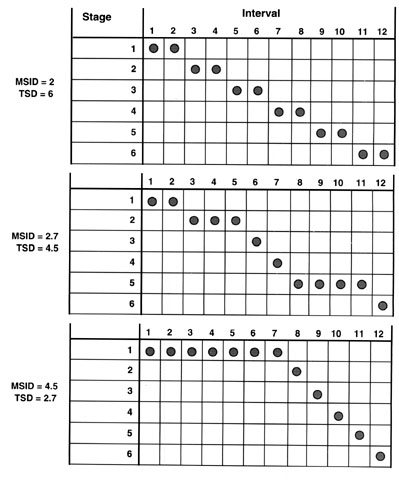
Fig. 3. Finite state diversity for the three avian species in Figure 1. Each column represents an interval in a temporal sequence of hypothetical life history stages (i.e. months in a year). The rows represent life history stages that vary according to species (see Fig. 1). The shaded circles indicate in which interval each life history stage is expressed by an individual in a given population. In the Rock Dove (top panel) there are two life history stages with relatively long durations and considerable overlap. MSID is high and TSD low. In the White-crowned Sparrow there are more life history stages with shorter durations and varying degrees of overlap. Here the MSID and TSD values are similar. In the Rock Ptarmigan, there are seven life history stages with some overlap. Now the MSID value is less than TSD. See text for details.
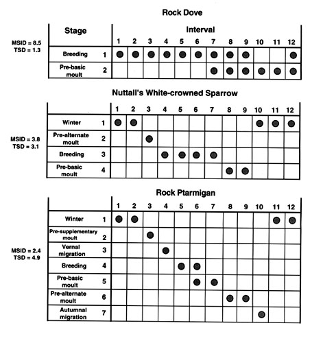
Fig. 4. A comparison of mean stage interval diversity calculated by the Shannon or Brillouin indices in relation to life history stages (phenotypic stages) in various avian taxa and populations. See legend for Fig. 5 for list of species. Values from the two methods are super-imposed.
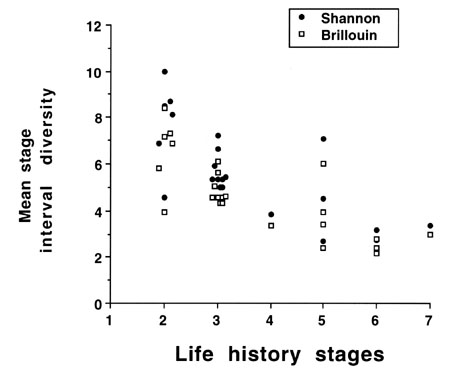
Fig. 5. Mean stage interval diversity (upper panel) and temporal stage diversity (lower panel), in relation to phenotypic stages (life history stages) of several taxa and sub-populations. These diversities were calculated from the Shannon index. Data were compiled from the following species: Masked Booby, Sula dactylatra, (Anderson 1992); Smith's Longspur, Calcarius pictus, (Briskie 1992); European Starling, Sturnus vulgaris, (Cabe 1992). Sooty Tern, Sterna fuscata, (Chapin 1954); Semipalmated Sandpiper, Calidris pusilla, (Gratto-Trevor 1992); Rock Ptarmigan, Lagopus mutus, (Holder & Montgomerie 1992); Rock Dove, Columba livia, (Johnston 1992); House Sparrow, Passer domesticus, (Lowther & Cink 1992); Cassin's Auklet, Ptychoramphus aleutica, (Manuwal & Thoresen 1992); Rufous-collared Sparrow, Zonotrichia capensis, (Miller 1962); Inca Dove, Scardafella inca, (Mueller 1992); Laysan Albatross, Diomedea immutabilis, (Whittow 1992); White-browed Sparrow Weaver, Plocepasser mahali, (Wingfield et al. 1991); Western Gull, Larus occidentalis wymani, (Wingfield et al. 1982); Zebra Finch, Poephila guttata, (Zann et al. 1995); Red Crossbill, Loxia curvirostra, (Hahn 1993); Snow Bunting, Plectrophenax nivalis (Romero et al. 1998); and several populations of White-crowned Sparrow, Zonotrichia leucophrys, and Song Sparrow, Melospiza melodia (Blanchard 1941; Blanchard & Erickson 1949; Mewaldt & King 1977); Wingfield & Farner 1978a,b; Wingfield & Hahn 1994).
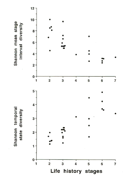
Fig. 6. Mean stage interval diversity and temporal stage diversity in relation to the number of life history stages in a sub-family of passerines (Emberizinae). See legend for Fig. 5 for species and references.
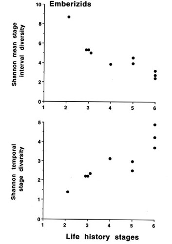
Fig. 7. Mean stage interval diversity and temporal stage diversity in relation to the number of phenotypic stages within a single genus, Zonotrichia. Taxa are: Z. capensis; Z. leucophrys gambelii; Z.l. nuttallii; Z.l. pugetensis, and Z.l. oriantha. See legend for Fig. 5 for references.
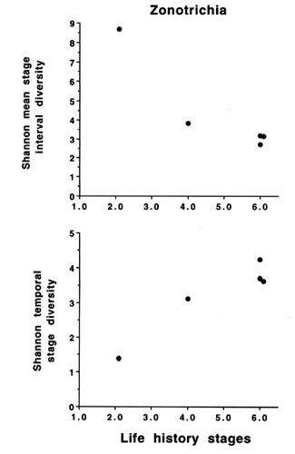
Fig. 8. Connectivity of different sub-stages within specific life history stages of the migratory White-crowned Sparrow, Zonotrichia leucophrys gambelii. Note that the sub-stages in each life history stage are unique. Even when some stages appear to be expressed in more than one life history stage (e.g. territorial behaviour in the breeding and winter stages), it is proposed that they are different in context and have separate control mechanisms. From Jacobs 1996.
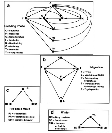
Fig. 9. Connectivity of sub-stages within the breeding life history stage from different taxa. Note that although the number of sub-stages in single-brooded and double-brooded populations may be the same, their connectivity differs because double-brooded species can revert back to the sexual phase after one set of young has become independent. From Jacobs 1996.
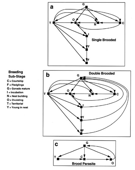
Fig. 10. Connectivity of sub-stages within the breeding life history stage within a population of, for example, cooperatively breeding birds. Breeding females show the full repertoire of sub-stages whereas breeding males may show only the sexual sub-stages. Conversely, non-breeding birds that are 'helpers-at-the-nest' may express parental sub-stages but no sexual sub-stages. From Jacobs 1996.
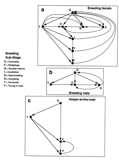
Fig. 11. Effects of experience of captive conditions on ovarian development in the first spring of female Song Sparrows, Melospiza melodia melodia. Hand raised females were captured from the same population as wild females. The hand raised birds were raised to independence in captive conditions and weaned onto laboratory chow. Wild females were captured after they had reached independence under natural conditions and then held over winter in captive conditions and fed laboratory chow. All birds were exposed to identical conditions of spring in their second year. Difference significant using Student's T test.