S06.3: Two-tier populations: Territory holders versus the rest
Steven E. Piper1 & Terry B. Oatley2
1Forest Biodiversity Programme, Department of Zoology and Entomology, University of Natal, Private Bag X01 Scottsville 3209 Pietermaritzburg, KwaZulu-Natal, South Africa, e-mail PiperS@zoology.unp.ac.za; 2Avian Demography Unit, Statistical Sciences Department, University of Cape Town, Private Bag, Rondebosch 7700 Western Cape, South Africa.
Piper, S.E. & Oatley, T.B. 1999. Two-tier populations: Territory holders versus the rest. In: Adams, N.J. & Slotow, R.H. (eds) Proc. 22 Int. Ornithol. Congr., Durban: 306-324. Johannesburg: BirdLife South Africa.
The current demographic theories of forest passerine demography are reviewed. While it is now accepted that passerines of the southern temperate zones have demographic patterns which are closer to those of tropical passerines no cogent reasons are presented for this. It is suggested that two factors may be responsible for these now well established life history traits: large-scale environmental variations (e.g. droughts and the El Niño Southern Oscillation phenomenon) and the holding of permanent all-purpose territories. In this paper we examine in detail the implications that permanent territories have for demography. We studied two species of forest passerines in the sub-tropical forests of South Africa for over twenty years, viz.: Starred Robin Pogonocichla stellata and Longtailed Wagtail Motacilla clara. Territory holders were fitted with unique permutations of colour-rings and individuals were followed for up to 11 years. Where possible their offspring were also marked and monitored. We found that territory-holders were very long-lived and often held one territory continuously for life and in some cases for up to a decade. There are no plumage differences between males and females (though males may have longer wings and tails by about 2 to 5 mm) and both males and females can hold a territory on the death of their partner and secure a replacement. Survival rates for territory holders varied from 70 to 85% p.a.- truly remarkable for birds of only 20 g (by comparison with northern temperate passerines). There is considerable year-to-year variation in the production of fledglings (up to ± 50%) but overall the productivity (typically 1.5 to 1.7 fledglings per pair p.a.) far exceeds the number needed to replace the breeding segment of the population. Fledglings joining the non-breeding segment of the population ‘float’ between the permanent territories for a number of years before finding a vacant territory, if ever. By comparison with species which select breeding territories anew each year, species in which the territories are held permanently differ in a number of respects and three testable predictions are motivated: (1) The proportion of fledglings that never recruit to the breeding population is higher. (2) The asymmetries in lifetime reproductive success are lower. (3) Non-breeders have a lower survival rate and a shorter life expectancy. Lastly, we caution against the use of capture-recapture/recovery data for estimating survival because this results in a pooled estimate of the two segments of the population and under-estimates both the survival and longevity of territory-holders.
INTRODUCTION
For nearly thirty years after the Second World War when David Lack conducted his pioneering studies of the life-history traits of birds, especially passerines (see Lack 1954), it was generally believed that the demography of passerines was a function of latitude only. It has been suggested that this old orthodoxy held because most passerines had at that time been studied in northern temperate climes (Skutch 1985). The first intimation that this orthodoxy might not hold, at least for Australian passerines, came from a comparison of longevity of a number of Australian passerines with northern temperate species (Fry 1980). This was followed by a comparison of clutch sizes between passerines in the Neotropics with those in North America (Skutch 1985) as well as a comparison of Australian passerines with those in North Africa (Yom Tov 1987).
From Lack’s studies, in which it was shown that clutch size increased with latitude (Lack 1954), it is to be expected that in the tropics passerines should have the smallest clutches and concomitant with this the highest survival rates. This has now been shown convincingly (see Johnson, Peach, Gregory and White 1997). Surprisingly it has been found that a number of passerines in the southern temperate zones have demographic parameters and life history traits much more like those of tropical zones (see extensive review of Australian, New Zealand and South African passerines in Rowley & Russel 1991). All else being equal, it is to be expected that passerines of southern temperate zones should have demographic parameters similar to those of north temperate zones at the same latitudes and of the same ecological niches and habitats (ibid.). Evidence has been accumulating since Rowley and Russel’s wide-ranging review (e.g. Martin 1996), but no suggestions have been advanced to account for these differences.
It is suggested that two factors may be invoked to explain these differences. Firstly, the passerines of the southern temperate zones have evolved in a hemisphere whose climate is currently dominated by frequent and unpredictable droughts as well as the El Niño Southern Oscillation (ENSO) phenomenon. Secondly, many more passerines in southern temperate climes hold permanent all-purpose territories than do species of similar ecological niche and habitat in northern temperate climes.
Evidence has been presented that ENSO has had a significant influence on the evolution of body size and metabolic parameters of mammals in the Southern Hemisphere (Lovegrove in press). We suggest that the possible effects of ENSO on the evolution of life history parameters of southern temperate zone passerines should be investigated further.
While it not possible to present an exact estimate of the proportion of fully and partially migratory passerines in northern temperate zones, it is clear that it is very much higher than that in southern temperate zones of the same latitude. For Australia it is possible to argue that its long and complete isolation, firstly from Gondwanaland and secondly from Asia, has meant that the majority of its ‘old’ passerines (sensu stricto Rowley & Russel 1991) evolved in a situation in which intercontinental migration was just not possible. In fact very few Australian passerines are migratory (ibid.). Because a large proportion of passerines are non-migratory it is to be expected that a higher number of species will have individuals which hold permanent territories. In so far as we can tell the demographic consequences of permanent territories held year-round have not been investigated (but see Sutherland 1996).
Clearly there is likely to be a continuum between those species in which territories are contested anew each year at the start of the breeding season through to those in which they are held permanently (i.e. ‘for life’ in common parlance). If a species is non-migratory and the territories are not permanent then it is likely that the demography will be little different from that of a fully migratory species except that the turnover of adults is likely to be lower because there are no losses ascribable to migration.
A species in which birds permanently occupy year-round exclusive territories (i.e. type ‘A’, Hinde 1956) is likely to differ in its demography from one in which territories are occupied anew at the start of the breeding season. The following differences are suggested, based on a population in which the breeders hold permanent, all-purpose territories.
(1) The proportion of fledglings that never recruit to the breeding population is likely to be higher.
(2) There is likely to be a lower asymmetry in the lifetime reproductive success (LRS) between individuals.
(3) The non-breeders (i.e. floaters) are likely to have a lower survival rate and hence a lower life expectancy.
The aim of this paper is to build a general mathematical model of passerine demography and use it to model our two study species so that we can motivate these testable predictions.
METHODS
The Starred Robin Pogonocichla stellata was studied in the mist-belt forests of KwaZulu-Natal at three sites.
(1) Kilgobbin Forest (29°29’S; 30°03’E) from 1953 to 1956 and from 1963 to 1978.
(2) Winterskloof (29°35’S; 30°18’E) from 1963 to 1973.
(3) Two Streams (29°18’S; 30°24’E) from 1975 to 1978.
Demographic parameters were estimated from the study of colour-ringed birds while breeding was studied by direct observation (Oatley 1982a, b, c). Other populations in Africa were studied opportunistically for limited periods (Oatley 1982a). All the robins of Africa have recently been reviewed (Oatley 1998).
The Longtailed Wagtail Motacilla clara was studied along the Palmiet River (29°49’S; 30°55’E) just outside the port city of Durban, also in the Province of KwaZulu-Natal from October 1976 to date. The data used in this analysis come from the period 1 August 1986 to 31 July 1998. Demographic parameters were estimated from the study of colour-ringed birds (Piper & Schultz 1988, 1989) while breeding was studied by direct observation (Piper 1989).
Models of passerine demography
A generalised model is constructed for a passerine species that can be counted once a year at the end of the breeding season. The model is based on a set of finite difference equations in which the four segments of the population are tracked: fledglings, sub-adults (for Starred Robin), non-breeders and territorial breeders. This model is flexible in that it can be adapted to a number of different circumstances, e.g. birds may breed at age one, or only at age two etc. To formulate the model the following assumptions are made.
(1) The population is made up of four stages: fledglings, sub-adults (for Starred Robin), non-breeders and breeders.
(2) The population is counted each year on 1st January when the (Austral) breeding season has come to an end.
(3) The population is closed, or at least all emigration is permanent.
(4) The population is at equilibrium: the population size is constant and the age structure stable.
The terms used in the equations below are defined (Table 1). The first model presented is for the Longtailed Wagtail and then this is modified for the Starred Robin and subsequent models.
Model of Longtailed Wagtail
If the population is at equilibrium then it is possible to perform a ‘mass balance’ on each of the three stages, i.e. breeding adults (nBR), non-breeders (nNB) and fledglings (nFL) and this yields the following three equations (Fig. 1). A complete list of symbols is provided in Table 1.
nBR = pBR * nBR + pFL_BR * nFL + pNB_BR * nNB: Eqn. 1
nNB = pFL_NB * nFL + pNB * nNB: Eqn. 2
nFL = F * nBR: Eqn. 3
In this model there are six demographic parameters that will have to be estimated before the population can be modelled. To make this model more tractable the following simplifying assumptions are made.
(5) The probability of a fledgling being recruited to the breeding population is assumed to be equal to that of a non-breeder.
pFL_BR = pNB_BR: Eqn. 4
(6) The survival rate of fledglings is assumed equal to that of non-breeders.
(pFL_BR + pFL_NB) = (pNB_BR + pNB)
Substituting equation 4 in to this yields the following equation.
pFL_NB = pNB: Eqn. 5
Using the above it is possible to simplify equations 1 and 2 to yield:
nBR = pBR * nBR + pNB_BR*(nFL + nNB): Eqn. 6
nNB = pNB*(nFL + nNB): Eqn. 7
This equation may be re-arranged to yield an estimate of the proportion of non-breeders in one year that remain non-breeders in the next (pNB).
pNB = nNB/(nFL + nNB): Eqn. 8
(7) For the sake of convenience the number of breeders (nBR) is scaled to unity.
nBR = 1: Eqn. 9
Using the above in equation 6 yields the following simplified equation.
(1-pBR) = pNB_BR*(nFL + nNB): Eqn. 10
The implication of equation 10 is that the loss of breeders is made up from recruitment from fledglings and non-breeders. Re-arranging this equation yields the following relationship.
nNB = (1-pBR)/pNB_BR – nFL: Eqn. 11
Using equation 9 reduces equation 3 to the following:
nFL = F: Eqn. 12
Model of the Starred Robin
Fledgling Starred Robins moult into a cryptic olive plumage for about 12 months and so are unable to breed in their first year, thus it is necessary to introduce an extra age-class into the model: sub-adults. Equations 1 and 2 need to be modified as shown below in equations 13 and 14. Equation 15 is added to account for the new age-class. Equation 3 is retained unaltered but is renumbered equation 16 (Fig. 2).
nBR = pBR * nBR + pSA_BR * nSA + pNB_BR * nNB: Eqn. 13
nNB = pSA_NB * nSA + pNB * nNB: Eqn. 14
nSA = pFL_SA * nFL: Eqn. 15
nFL = F * nBR: Eqn. 16
Use assumption 7, i.e. equation 9, to scale the number of breeding adults to unity. Thus equations 13 and 16 reduce to the following:
(1 – pBR) = pSA_BR * nSA + pNB_BR * nNB: Eqn. 17
nFL = F: Eqn. 18
The implication of equation 17 is that the loss of breeders is made up from recruitment from sub-adults and non-breeders a year later. This model can be simplified by the use of the following assumptions.
(8) The probability of a sub-adult recruited to the breeding population is assumed to be equal to that of a non-breeder.
pSA_BR = pNB_BR: Eqn. 19
(9) The survival rate of sub-adults is assumed equal to that of non-breeders.
(pSA_BR + pSA_NB) = (pNB_BR + pNB)
Substituting equation 19 in to this yields the following equation:
pSA_NB = pNB: Eqn. 20
Using equation 19 in equation 17 yields equation 21.
nNB = (1 – pBR)/ pNB_BR - nSA
This can be re-arranged to yield:
pNB_BR = (1 – pBR)/ (nNB + nSA): Eqn. 21
Using equation 20 in equation 14 yields:
pNB = nNB/(nNB + nSA): Eqn. 22
Nulls models
In order to test the effects of permanent territories it is necessary to create null models which are in every respect identical to the species’ models except that they allow all individuals to compete equally for territories at the start of each successive breeding season.
Null model for Longtailed Wagtail
This model is identical to that formulated above (Fig. 1) except that a new linkage has been added: birds breeding this year may become non-breeders next year. The fundamental equations include equation 1 and 3 from above but equation 2 is altered as follows:
nNB = pBR_NB * nBR + pFL_NB * nFL + pNB * nNB: Eqn. 23
Simplifying assumptions: Null model for Longtailed Wagtail
(10) The probability of a non-breeder being recruited to the breeding population is assumed to be equal to that of a breeder.
pNB_BR = pBR: Eqn. 24
(11) The survival rate of non-breeders is assumed equal to that of breeders.
(pNB_BR + pNB) = (pBR_NB + pBR)
Substituting equation 24 in to this yields the following equation:
pBR_NB = pNB: Eqn. 25
(12) The survival rate of adults (i.e. birds after their first year) is assumed to be equal to the average survival rate of adults in the Longtailed Wagtail model above.
(pBR_NB + pBR) = p_LTW: Eqn. 26
Where p_LTW is the weighted average of p_BR and (pNB+pNB_BR) in the Longtailed wagtail model using nBR and nNB as the weights.
Using equations 24 and 25 it is possible to simplify equations 1 and 23 to yield:
nBR = pBR * (nBR + nNB) + pFL_BR * nFL: Eqn. 27
nNB = pBR_NB * (nBR + nNB) + pFL_NB * nFL: Eqn. 28
Adding these two equations yields:
(nBR+ nNB) = (pBR+ pBR_NB)* (nBR + nNB) + (pFL_BR+ pFL_NB) * nFL
(nBR+ nNB) * (1 – [pBR+ pBR_NB]) = (pFL_BR+ pFL_NB) * nFL
Using equation 26 this reduces to the following:
(nBR + nNB) * (1 - p_LTW) = (pFL_BR+ pFL_NB) * nFL
From this it follows that:
(pFL_BR+ pFL_NB) = (nBR + nNB) * (1 - p_LTW)/nFL: Eqn. 29
Equation 29 provides an estimate for the survival rate of fledglings.
Null model for male Starred Robins (nNB=0.1)
This model is identical to that formulated above (Fig. 2) except that a new linkage has been added: birds breeding this year may become non-breeders next year. The fundamental equations include equations 13, 15 and 16 from above but equation 14 is altered as follows:
nNB = pBR_NB * nBR + pSA_NB * nSA + pNB * nNB: Eqn. 30
Simplifying assumptions: Null model for male Starred Robin (nNB=0.1)
Assumptions 10 and 11 from above are used along with equations 24 and 25.
(13). In the null model the survival rate of adults (i.e. after sub-adults have moulted into their adult plumage) is assumed to be equal to the average survival rate of adults in the Starred Robin model above.
(pBR_NB + pBR) = p_SR-C: Eqn. 31
Where p_SR-C is the weighted average of p_BR and (pNB+pNB_BR) in the Starred Robin model (nNB=0.1, Fig. 3) using nBR and nNB as the weights.
Using equations 24 and 25 it is possible to simplify equations 13 and 30 to yield.
nBR = pBR * (nBR+ nNB) + pSA_BR * nSA: Eqn. 32
PnNB = pBR_NB * (nBR + nNB) + pSA_NB * nSA: Eqn. 33
Adding these two equations yields:
(nBR+ nNB)= (pBR+ pBR_NB) * (nBR + nNB) + (pSA_BR+ pSA_NB) * nSA
(nBR+ nNB) * (1 – [pBR+ pBR_NB]) = (pSA_BR+ pSA_NB) * nSA
Using equation 31 this reduces to the following:
(nBR + nNB) * (1 - p_SR-C) = (pSA_BR+ pSA_NB) * nSA
From this it follows that:
(pSA_BR+ pSA_NB) = (nBR + nNB) * (1 - p_SR-C)/nSA: Eqn. 34
Equation 34 provides an estimate for the survival rate of sub-adults.
Variation in potential lifetime reproductive success (LRS)
If territories are permanent then non-breeders have to wait for ‘dead men’s shoes’ and are likely to have a lower reproductive output than if territories are contested anew each breeding season. To test this we have constructed two null models that correspond to each species and differ from the species models only in respect of territory permanence. By comparing the lifetime reproductive success (LRS) of birds in each of the species models with those in the corresponding null model we are able to quantify one of the consequences of holding permanent territories. To do this the age at which birds of each species first breed is evaluated and then the average productivity is computed.
Age first breed: Longtailed Wagtail
The proportion of birds breeding in their first year is pFL_BR (Fig. 1). The proportion breeding in their second year is the product of the proportion that survived to become non-breeders in their first year and then joined the breeding population in their second year, i.e. pFL_NB * pNB_BR. It is possible to compute the probabilities for all subsequent years in a similar fashion (Table 2).
Age first breed: Starred Robin
The model for the Starred Robin differs from that of the Longtailed Wagtail in respect of a non-breeding stage which prevents them from breeding in the first year. Based on direct observation it is known that there are very few, if any, female floaters (nNB) in the population (Oatley 1982c). Hence a model has been formulated in which nNB=0 and a direct consequence of this is that new individuals can only be recruited to the breeding adult population in their second year and the proportion of females recruited is pFL_SA * pSA_BR (Fig. 2). Two models have been formulated for males (Fig. 3 and Fig. 4), i.e. for nNB = 0 and 0.01 respectively and the proportions joining the breeding population have also been computed (Table 2).
Lifetime productivity
In the first year in which an individual breeds its fecundity is F, measured as female offspring per breeding female (or equivalently per breeding pair, assuming a sex ratio of 50:50). Having bred once year proportion surviving to breed in the second year is pBR where the output will be (F * pBR), thus the lifetime output of a bird, once recruited to the breeding population is (summing an infinite series):
F + F* pBR + F*(pBR)2 + F*(pBR)3 + … = F(1+ pBR + (pBR)2 + (pBR)3+ …)= F/(1-pBR)
RESULTS
Estimates of parameters Longtailed Wagtail
Reasonable values may be provided for the following demographic parameters. The number of breeding adults (nBR) has been arbitrarily scaled to unity (assumption 7, equation 9). The average fecundity (F) is approximately 0.85 female fledglings per female p.a. (Piper 1989, pers obs. SEP). The survival rate of breeding adults (pBR) was as high as 0.80 in 1986-7 but has dropped steadily over the years to about 0.65 (Piper 1994, pers obs. SEP). For comparison with the null model below it will be assumed that pBR=0.75.
Because all or nearly all territory holders are colour-ringed in the study site it is possible to identify floaters as un-ringed birds, or as ringed birds that do not have a territory. From direct counts of floaters it is estimated that there are at most one or two floaters passing through the study site which contains 11 or 12 pairs. If it assumed that the sex-ratio of the floaters is 50:50 then there will be between 1/11 to 0.5/12 non-breeding females per breeding adult female, i.e. nBR = 0.0417 to 0.0909.
If it is known what proportion of breeders survive (pBR) and what the fecundity (F) is then it is possible to use equation 11 to investigate the relationship between the number of non-breeders (nNB) and the rate at which they are recruited to the breeding population (pNB_BR). Thus for pBR=0.75, F=0.85 and 0.0417<nBR<0.0909 it is possible to estimate that the proportion of non-breeders recruited (pNB_BR) is likely to be about 0.2657 (Fig. 5). In fact, in the limit as the number of non-breeders tends to zero it is possible to rewrite equation 11 as pNB_BR = (1-pBR)/nFL and in this case pNB_BR will be 0.294 which is clearly an upper limit.
Given estimates of the number of fledglings (0.85) and the number of non-breeders (0.0417< nBR< 0.0909) it is possible to compute the proportion of non-breeders which survive to be non-breeders in the next year (pNB) from equation 8. Thus 0.047< pNB< 0.0966 and using a recruitment rate of pNB_BR=0.2657 it follows that the survival rate of non-breeders (pNB_BR + pNB) is in the range 0.322 to 0.3623 (Fig. 6). Final parameter estimates are summarised for the Longtailed Wagtail (Fig. 1).
Starred Robin Reasonable values may be provided for the following demographic parameters. The number of breeding adults (nBR) has been arbitrarily scaled to unity (assumption 7, equation 9). The average fecundity (F) is computed as the ratio of 91 fledglings produced from 60 nesting attempts; assuming a sex ratio of 50:50 and knowing that Starred Robins breed once p.a. it may be estimated that F = 91/(60*2) = 0.758 (Oatley 1982c). The survival rates of sub-adult females was estimated from the ratio 11/14 and of adult females from the ratio 76/100 and because these two ratios are not statistically different (c 2 test, p>0.1) they may be combined, i.e. female survival = 87/114 = 0.763 (ibid.). The survival rates of sub-adult males was much lower at 0.556 while that for adult males was higher, 0.837 (ibid.)
Because all or nearly all territory holders were colour-ringed in the study site it was possible to identify floaters as un-ringed birds, or as ringed birds that did not have a territory. Adult female floaters were never seen though they may have existed. Adult male floaters were seen occasionally during the breeding season though these may just have been males seeking extra-pair copulations. However, a male that died during the breeding season was replaced and this hints at the presence of available floaters.
For female Starred Robins no floaters in breeding plumage were every seen and so as a limiting case it may be assumed that nNB @ 0. Using this approximation it is possible to rewrite equation 17 as pSA_BR = (1 – pBR)/ nSA = (1-0.763)/0.579, hence pSA_BR = 0.409 (Fig. 2).
For male Starred Robins the situation is slightly more complicated as floaters in adult breeding plumage were seen during the breeding season, though they were few in number (Oatley 1982c). The number of male fledglings is 0.758 (from equation 16) while the number of male sub-adults is 0.421 (from equation 15). Arguing as above (equation 17) the limiting value of pSA_BR for males (i.e. nNB = 0) is (1 – pBR)/ nSA = (1-0.837)/0.421 i.e. pSA_BR = 0.387 (Fig. 4).
While it is not known exactly how many non-breeding adult male floaters there are in the system it is likely, to at least an order of magnitude that they are somewhere in the range 0 to 0.1 (i.e. measured as male floaters per breeding adult male). The relationship between the number of non-breeders in adult plumage (nNB) and their recruitment rate (pNB_BR) may be investigated via equation 21. Plotting both it is seen that for 0<nNB<0.1 the recruitment rate will lie in the range 0.313< pNB_BR< 0.387 (Fig. 7). It is possible to estimate the proportion of non-breeders who will be non-breeders a year later (pNB) as a function of the number of non-breeders (nNB) from equation 22. Plotting these two quantities shows that for 0<nNB< 0.1 the limits on pNB will be 0<pNB<0.192 (Fig. 3).
Null model: Longtailed Wagtail
Given the average survival of adults (p_LTW) it is possible to compute the survival rate of fledglings in the null model using equation 29. An estimate of p_LTW is (0.75 + 0.0909*0.3623689)/(1 + 0.0909) = 0.7176932. The estimate of fledgling survival is almost identical to that for the permanent territory model so it seems sensible to use the same value of 0.2657 for pFL_BR in both models. Using this value of pFL_BR it is possible to estimate pBR = 0.7096 from equation 27. Subtracting pFL_BR from the estimate of fledgling survival yields pFL_NB = 0.0966 and this may be substituted into equation 28 to get an estimate of 0.0081 for pBR_NB (Fig. 8). From this it may be seen that the survival rate of non-breeders is 0.7177 (=pNB_BR + pNB, Fig. 8) and this is much higher than in the model of permanent territory holders where it is 0.2657 + 0.0996 = 0.3623 (Fig. 1). In fact it is nearly half!
Null model: male Starred Robin (nNB=0.1)
Given the average survival of adults (p_SR-C) it is possible to compute the survival rate of sub-adults in the null model using equation 34. An estimate of p_SR-C is (0.837 + 0.1*(0.3128599+0.1919386)/(1 + 0.1) = 0.5047985. The estimate of sub-adult survival is identical to that for the permanent territory model and it seems sensible to use the same value of 0.3128599 for pSA_BR in both models. Using this value of pSA_BR it is possible to estimate pBR = 0.7893509 from equation 32. Subtracting pSA_BR from the estimate of sub-adult survival yields pSA_NB = 0.1919386 and this may be substituted into equation 33 to get an estimate of 0.0174490 for pBR_NB (Fig. 9). From this it may be seen that the survival rate of non-breeders is 0.8067999 (=pNB_BR + pNB, Fig. 9) and this is much higher than in the model of permanent territory holders where it is (0.3128599 + 0.1919386) = 0.5047985 (Fig. 3). In fact it is lower by 37%
Variations in potential lifetime reproductive success: Longtailed Wagtail
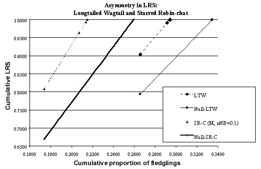
Using the formula developed above (Table 2) and estimates of the population parameters (Fig. 1 & Fig. 8) it is possible to compute the proportion of fledglings which breed for the first time at age 1, 2, 3 etc. (Fig. 10). The proportion who breed for the first time at the end of their first year is almost the same for permanent territory and null models (26.57%) but is higher for the null model in the second year (6.85% versus 2.57%) but lower in all subsequent years. A similar pattern holds for LRS (Fig. 11). The asymmetry in LRS may be seen by plotting the cumulative LRS as a function of the cumulative number of fledglings recruited to the breeding population (Fig. 12). From this it may be seen that a lower proportion of fledglings are recruited to the population with permanent territories than in null model (i.e. 29.41% versus 33.48%). For the model of permanent territory holders, birds breeding at age one have a LRS of 0.9034 while for the null model its is 0.7936. Thus birds in the population of permanent territory holders have a lower variation in potential LRS.
Variations in potential lifetime reproductive success: male Starred Robin (nNB=0.1)
Using the formula developed above (Table 2) and estimates of the population parameters (Fig. 3 & Fig. 9) it is possible to compute the proportion of fledglings which breed for the first time at age 2, 3, 4 etc. (Fig. 10) – of course none breed at the end of their first year. The proportion who breed for the first time at the end of their second year is almost the same for permanent territory and null models (17.39%) but is higher for the null model in the third year (8.42% versus 3.34%) but lower in all subsequent years. A similar pattern holds for LRS (Fig. 11). The asymmetry in LRS may be seen by plotting the cumulative LRS as a function of the cumulative number of fledglings recruited to the breeding population (Fig. 12). From this it may be seen that a lower proportion of fledglings are recruited to the population with permanent territories than in null model (i.e. 21.52% versus 25.95%). For the model of permanent territory holders, birds breeding at age two have a LRS of 0.8086 while for the null model its is 0.6699. Thus birds in the population of permanent territory holders have a lower variation in potential LRS.
DISCUSSION
While it is generally recognised that passerines of the ‘southern temperate zones’ have life history traits more similar to those of tropical species than species of northern temperate zones (at the same latitude and in the same ecological niche and habitat type) no acceptable reasons for this have yet been advanced (Rowley & Russel 1991). It should be noted, however, that widespread reference to the extra-tropical portions of southern continents as ‘southern temperate zones’ is misleading, since a climatic regime similar to that of the northern temperate zone does not occur anywhere in the southern hemisphere (Darlington 1965). We should not, therefore, expect that species traits of extra-tropical southern hemisphere passerines should be the same as those of their northern temperate zone counterparts, even when exclusively extra-tropical distributions would qualify them as ‘temperate’ species.
We suggest that holding a permanent, all-year and life-long territory is an important life-history trait differentiating southern hemisphere passerines from those of the northern hemisphere. To give substance to our hypothesis we have built models of the population dynamics of our two study species. In these models the demographic difference between the territory and floating sections of the population are made explicit. The models have been used to provide estimates of the demographic parameters and these have been compared with estimates from the null models. The null models differ only in one respect: territories are not permanently held.
From a comparison of each species models with its corresponding null model it is possible to provide a quantitative evaluation of the three testable hypotheses provided above.
(1) The proportions of fledglings that recruit to the breeding population are 22% and 29% respectively for the Starred Robin and Longtailed Wagtail. These values jump to 26% and 33% in the null models, i.e. where territories are settled anew each year. These represent relative increases of 20.6% and 13.8% respectively.
(2) The potential LRS of the Starred Robin is lower in comparison with that of the null model (Fig. 12): 0.809 for the first age class in which breeding occurs (i.e. in the second year) versus 0.670 for the null model, a drop of 17%. For the Longtailed Wagtail the corresponding figures are 0.903 and 0.794, i.e. a drop of 12%. In other words, allowing competition for territories each year gives a few extra individuals the chance of contributing to the next generation.
(3) In populations with permanent territories it is more difficult for a fledgling to recruit to the breeding population and hence to survive. For the Starred Robin males (in the nNB=0.1 model) the survival rate non-breeders was 50.5% (Fig. 3) and this rose to 80.7% in the null model (Fig. 9). The corresponding change for Longtailed Wagtail was 36.23% to 71.8%. These represent increases of nearly 60% and 99% for the two species.
Thus we have shown that holding permanent territories does indeed impact upon a number of demographic parameters, most especially the survival of non-breeders.
As no floaters were ever seen for adult female component of the Starred Robin component of the population it is not possible to model the effect of permanent territories. In fact, this suggests that adult females could even be a limiting resource for the Starred Robin.
The parameters used in these models come from our own observations and field work and we can attest to their accuracy within the limitations of sample size. In both our studies we have been able to overcome partially the constraints of small sample size by collecting data over long periods (>20 years each). However, we have not been able to observe all parameters directly and some (e.g. survival of non-adults and recruitment) have had to be estimated from the models by making an assumption of equilibrium. We have no measure of how restrictive this assumption is nor do we know to what extent it impinges on our conclusions. Clearly to improve the quality of our models we need direct estimates of these two parameters, albeit that they are difficult to measure.
No model is better than its assumptions. It is probable that the most serious limitations of our model are the explicit and implicit assumptions of parameter constancy in space and time. While it is suspected that territories vary in quality and some years were clearly more productive than others we have no measures of these variations and have not included them in our models.
ACKNOWLEDGEMENTS
We thank all those persons who helped us in the field. The help of the staff of the Southern African Bird Ringing Unit (Safring) is gratefully acknowledged.
REFERENCES
Darlington, P.J. Jr. (1965). Biogeography of the southern end of the world. Harvard University Press: Cambridge.
Fry, C. H. (1980). Survival and longevity of among tropical land birds. Fourth Pan-African Ornithological Conference. (ed.) D. N. Johnson. Johannesburg: South African Ornithological Society: 334-43.
Hinde, R. A. (1956). The biological significance of the territories of birds. Ibis 98: 340-369.
Johnston, J. P., W. J. Peach, R. D. Gregory and S. A. White (1997). Survival rates of tropical and temperate passerines: a Trinidadian perspective. American Naturalist 150(6): 771-789.
Lack, D. (1954). The natural regulation of animal numbers. Oxford: Clarendon.
Martin, T. E. (1996). Life history evolution in tropical and south temperate birds: What do we realy know. Journal of avian biology 27(4): 263-272.
Oatley, T. B. (1982). The Starred Robin in Natal, Part 1: Behaviour, territory and habitat. Ostrich 53: 135-146.
Oatley, T. B. (1982). The Starred Robin in Natal, Part 2: Annual cycles and feeding ecology. Ostrich 53: 206-221.
Oatley, T. B. (1982). The Starred Robin in Natal, Part 3: Breeding, populations and plumages. Ostrich 53: 206-221.
Oatley, T. B. (1998). The robins of Africa. Randburg & Halfway House: Acorn Books & Russel Friedman Books.
Perrins, C. M. and T. R. Birkhead (1983). Avian ecology. Glasgow: Blackie.
Piper, S. E. (1989). Breeding biology of the Longtailed Wagtail Motacilla clara. Ostrich Supplement 14: 7-15.
Piper, S. E. (1994). Estimates of minimum survival rates for territorial, adult Longtailed Wagtails, Motacilla clara. Journal fur Ornithologie 135: 500.
Piper, S. E. and D. M. Schultz (1988). Monitoring territory, survival and breeding in the Longtailed Wagtail. Safring News 17(2): 65-76.
Piper, S. E. and D. M. Schultz (1989). Type, dimensionality and size of Longtailed Wagtail territories. Ostrich Supplement 14: 123-131.
Rowley, I. and E. Russell (1991). Demography of passerines in the temperate southern hemisphere. Bird population studies. (ed.) C. M. Perrins, J.-D. Lebreton and G. J. M. Hirons. Oxford: Oxford University Press: 22-44.
Skutch, A. F. (1985). Clutch size, nesting success, and predation on nests of neotropical birds, reviewed. Neotropical ornithology. (ed.) P. A. Buckley, M. S. Foster, E. A. Morton, R. S. Ridgely and F. G. Buckley: Ornithological Monographs. 36: 575-594.
Sutherland, W. J. (1996). From individual behaviour to population ecology. Oxford: Oxford University Press.
Yom-Tov, Y. (1987). The reproductive rates of Australian passerines. Australian Wildlife Research 14: 319-330.
Table 1. Parameter definition
Table 2. Age of first breeding: proportion that breed for the first time at each age
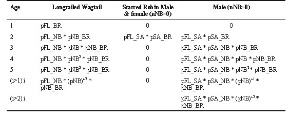
Fig. 1. Flow chart for the Longtailed Wagtail model (females only) with parameter estimates.
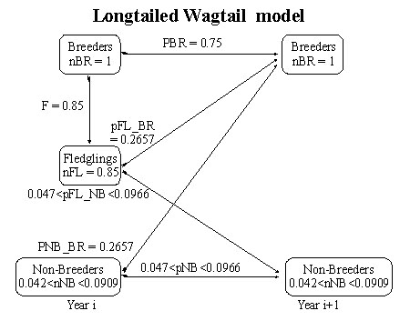
Fig. 2. Flow chart for the Starred Robin model (females only) with parameter estimates under the assumption that the number of non-breeding floaters (nNB) is close to zero.
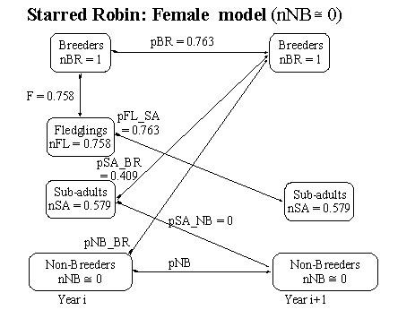
Fig. 3. Flow chart for the Starred Robin model (males only) with parameter estimates under the assumption that the number of non-breeding floaters (nNB) is estimated to lie in the range 0.0 < nNB< 0.1.
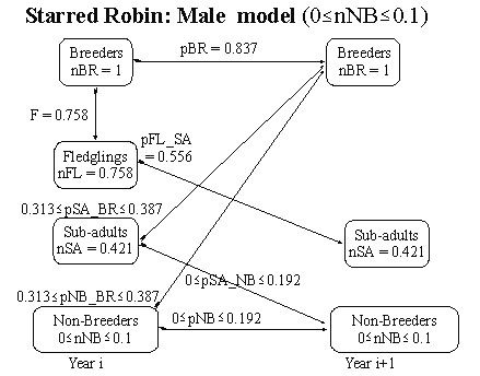
Fig. 4. Flow chart for the Starred Robin model (males only) with parameter estimates under the assumption that the number of non-breeding floaters (nNB) is effectively zero.
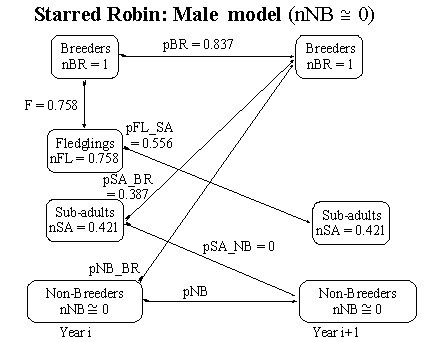
Fig. 5. The relationship between the number of non-breeders (nNB) and the proportion of non-breeders recruited to the breeding population (pNB_BR) as computed from equation 11 for the Longtailed Wagtail. Fecundity (F) is assumed to be 0.85 and equation 11 is evaluated for a range of survival rates. If the number of non-breeders (nNB) is set to zero then it is possible to compute the asymptotic values for pNB_BR and these are shown as crosses along the lower axis. The upper limit is the locus of those value of nNB and pNB_BR along which the survival rate of non-breeders (pNB_BR + pNB) is equal to the survival rate of breeders (pBR).
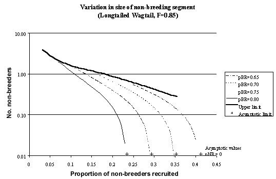
Fig. 6. The relationship between the survival rate of non-breeders (pNB_BR + pNB) and the number of non-breeders (nNB) as computed from equation 8 for the Longtailed Wagtail. Fecundity is assumed to be 0.85 and equation 8 is evaluated for a variety of survival rates.
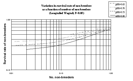
Fig. 7. The relationship between the number of non-breeders (nNB) and the proportion of non-breeders recruited to the breeding population (pNB_BR) as computed from equation 21 and the proportion of non-breeders who will be retained as non-breeders (pNB) as computed from equation 22 for Starred Robin males. Number of sub-adult males (nSA) is assumed to be 0.421 while the survival rate of breeding adults (pBR) is 0.837.
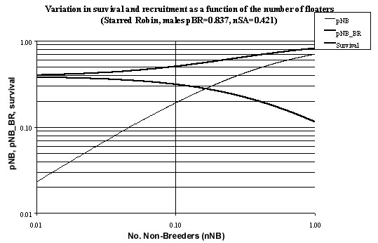
Fig. 8. Null model for the Longtailed Wagtail in which it is assumed that territories are not permanent.
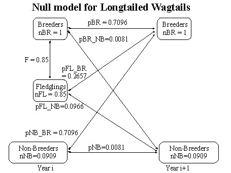
Fig. 9. Null model for the Starred Robin males (nNB =0.1) in which it is assumed that territories are not permanent.
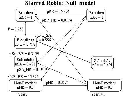
Fig. 10..Proportion of fledglings which first breed at a given age. Abbreviations: LTW = Longtailed Wagtail, standard model (Fig. 1); Null-LTW = Null model for the Longtailed Wagtail; SR-C (F) = Starred Robin, females (Fig. 2); SR-C (M, nNB=0) = Starred Robin, males (Fig. 4); SR-C (M, nNB=0.1) = Starred Robin, males (Fig. 3); Null-SR-C = Null model for Starred Robin, males (Fig. 9).
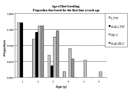
Fig. 11. Potential lifetime reproductive success of fledglings which first breed at a given age. Abbreviations: LTW = Longtailed Wagtail, standard model (Fig. 1); Null-LTW = Null model for the Longtailed Wagtail; SR-C (F) = Starred Robin, females (Fig. 2); SR-C (M, nNB=0) = Starred Robin, males (Fig. 4); SR-C (M, nNB=0.1) = Starred Robin, males (Fig. 3); Null-SR-C = Null model for Starred Robin, males (Fig. 9).
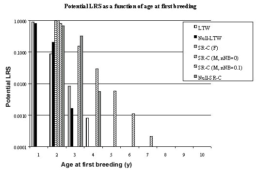
Fig. 12. Asymmetry in lifetime reproductive success. Abbreviations: LTW = Longtailed Wagtail, standard model (Fig. 1); Null-LTW = Null model for the Longtailed Wagtail; SR-C = Starred Robin, males nNB=0.1 (Fig. 3); Null-SR-C = Null model for Starred Robin, males (Fig. 9).